
You can also find this library at CRAN and download it directly from R and RStudio.
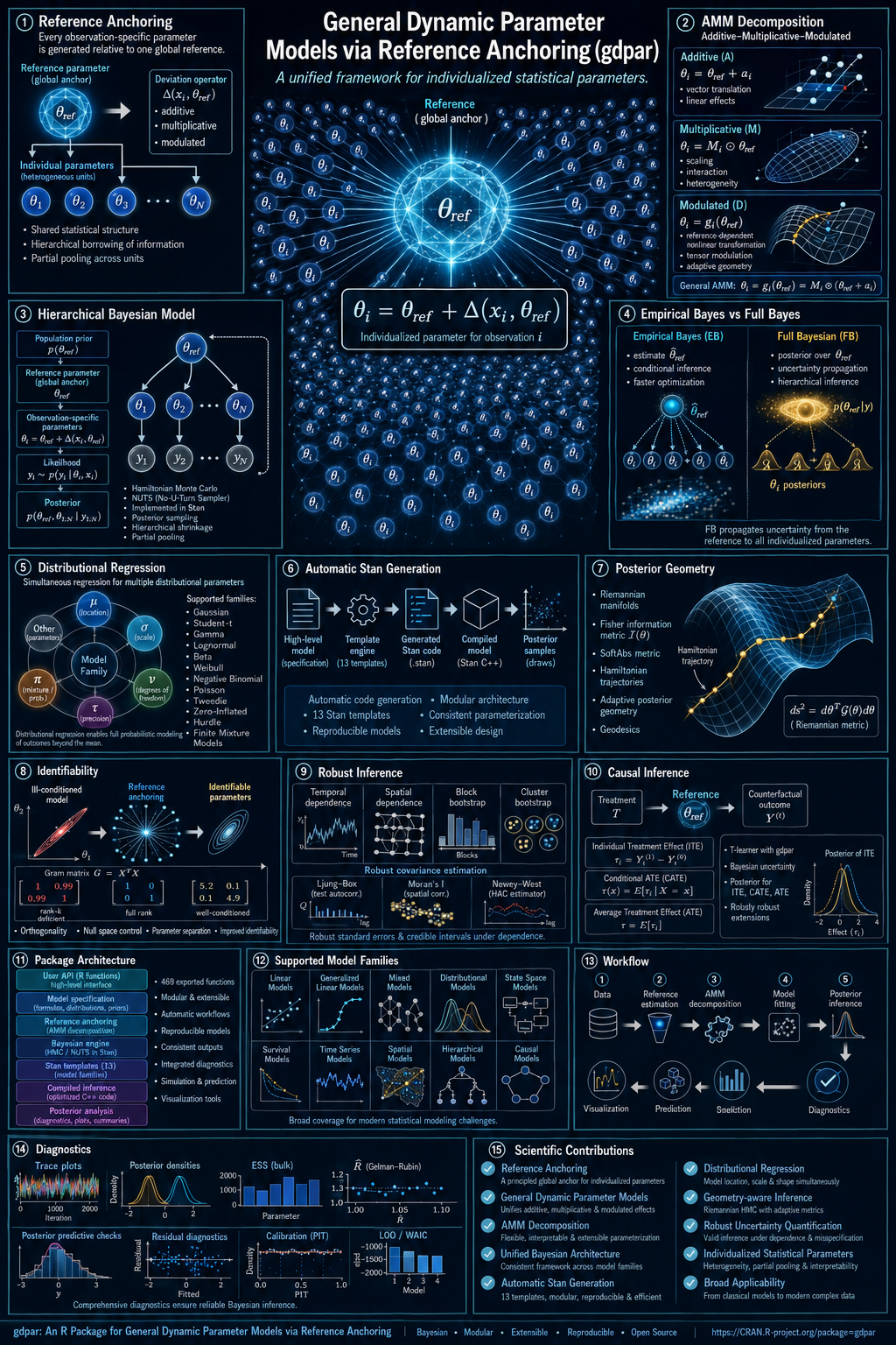
Also, we recommend viewing the mind map summary at the end of the article to better understand the relationship between the functions of the package.
LISTEN TO THIS POST AS A PODCAST:
ESCUCHA ESTA PUBLICACIÓN COMO PODCAST
Meet gdpar
In the fleeting calculus of a two-second decision—overtaking a car on a narrow road—the human brain performs a remarkable statistical trick. It does not build a model of the approaching driver from scratch. Instead, it retrieves a baseline: the average driver, representing typical reaction times and modal aggression. In a split second, it reads the specific signals of the actual driver—relative speed, vehicle type, micro-movements—and estimates how this specific driver deviates from the baseline. The decision to overtake emerges from that synthesis.
This cognitive recipe—population reference + individual deviation—is the philosophical bedrock of the R package gdpar (General Dynamic Parameter models via Reference Anchoring) by José Mauricio Gómez Julián. The package takes this intuition, formalizes it as a rigorous statistical decomposition, proves the conditions under which it is mathematically identifiable, ships a Stan-based Bayesian engine to estimate it, and layers on causal inference, geometry-adaptive sampling, and dependence-robust inference.
The Anatomy of Deviation
Every layer of gdpar is an elaboration of a single, elegant equation. For each observation $i$ with covariates $x_i$:
Read it as: the parameter of individual $i$ equals a population reference, plus a deviation that is itself a function of the individual’s covariates and of the reference itself.
That final clause is where the architecture pivots from classical statistics. The deviation $\Delta$ does not merely depend on who you are (your covariates $x_i$); it depends on what the reference is. If you transplant the model to a new population, the deviation function behaves differently because $\theta_{\text{ref}}$ is one of its arguments. This structural dependence is the defining feature of “reference anchoring.” It distinguishes gdpar from random-effects or varying-coefficient models, where the deviation is structurally separate from the reference.
So, what is the shape of $\Delta$? The package singles out a specific functional form called the Additive–Multiplicative–Modulated (AMM) decomposition:
Three mechanisms, cleanly separated and independently interpretable:
- $a(x)$ — A pure additive shift. Think of this as a traditional fixed-effect driven by covariates.
- $b(x)\odot\theta_{\text{ref}}$ — A covariate-dependent scaling of the reference (using the Hadamard/elementwise product). This is where “the deviation depends on the reference” enters multiplicatively.
- $W(\theta_{\text{ref}})\,x$ — Covariates are mixed through a matrix $W$ that is, itself, tuned by the reference. This is the explicit, structural reference-dependent channel.
Standard models drop out as special cases. Set $\Delta \equiv 0$ and you have fixed-effects regression. Set $W \equiv 0$ and you have a hierarchical model with multiplicative interaction. Set $b \equiv 0$ and you have a varying-coefficient model. The AMM is the smallest natural family that contains all three and elevates the reference to an active argument of the deviation.
The Three Estimation Engines
gdpar defines three complementary engines for estimating $\Delta$. Crucially, only one is executable in the current release—a deliberate choice to promise a mathematical scope that exceeds the executable surface, and to say so honestly.
| Path | Engine | Representation | Status |
|---|---|---|---|
| Path 1 | Hierarchical Bayesian (Stan) | Parametric AMM | ✅ Operational |
| Path 2 | Varying-coefficient (splines) | Smooth $\beta(z)$ | 🚧 Conceptual |
| Path 3 | Hypernetwork / Neural Net | Net generates $\theta_i$ | 🚧 Conceptual |
Paths 2 and 3 are documented to “reference grade”—full asymptotic theory (contraction rates, Bernstein–von Mises) is developed in the Wiki—but they abort with gdpar_unsupported_feature_error if invoked. Path 1 places priors on every component ($\theta_{\text{ref}}, a, b, W$) and samples the joint posterior with HMC, yielding native, full-posterior uncertainty.
A Tale of Two Posteriors: EB vs. FB
Within Path 1, gdpar offers two inferential regimes. Full Bayes (FB) via gdpar() samples the joint posterior, remaining most faithful to the cognitive analogy. Empirical Bayes (EB) via gdpar_eb() estimates the hyperparameters by maximizing a marginal likelihood via a Laplace approximation, then samples the remaining parameters conditionally.
The EB vs FB Comparator
Rather than forcing a choice, gdpar treats them as parallel routes. It ships a dedicated comparator, gdpar_compare_eb_fb(), which quantifies agreement on $\theta_{\text{ref}}$ and the reduced parameter vector $\xi$. The Wiki develops the theory to first-class depth: EB and FB lower-level posteriors agree asymptotically (Theorem 7A), while EB intervals under-cover by $O(n^{-1})$ (Proposition 7B). If you have ever wondered if EB is “good enough” for your data, gdpar lets you answer that empirically.
Distributional Regression: Every Parameter is a Slot
gdpar is not constrained to modeling the mean. A probability distribution has multiple parameters—location, scale, shape, tail index, zero-inflation probability—and each one can carry its own AMM decomposition. The package indexes these by $k = 1, \dots, K$:
The built-in roster covers Gaussian, Poisson, negative binomial, Bernoulli, Beta, Gamma, Student-$t$, Tweedie, ZIP, ZINB, and hurdle families. Zero-inflated and hurdle models receive an especially elegant treatment: both the zero-inflation probability $\pi_i$ and the count parameter $\theta_i$ are anchored to their respective references—a dual deviation design.
The Causal Bridge
Because the AMM form produces individual parameters, individual treatment effects emerge naturally. gdpar_causal_bridge() implements a T-learner: fit the anchored model separately under treatment and control, then read the conditional average treatment effect (CATE) at $x_i$ as the difference of the anchored individual predictions:
A second layer, gdpar_compare_meta_learners(), benchmarks the AMM-based learner against external meta-learners via pluggable adapters: grf::causal_forest on the R side and EconML’s CausalForestDML on the Python side (via reticulate). The framework’s causal claims are benchmarked, not asserted.
Mechanics & Clockwork
Several engineering decisions elevate gdpar from a theoretical exercise to a serious computational environment:
- Stan Code Generator: Composes programs from canonical pieces—AMM blocks for $p=1$ and $p \geq 1$, EB marginal/conditional blocks, distributional-$K$ blocks—selected by the resolved $(K, p, \text{family}, W, \text{parametrization}, \text{group})$. The $W$ basis supports B-splines with Stan-side Cox–de Boor evaluation, ensuring differentiability inside HMC.
- Identifiability Pre-flight: Before any sampling,
gdpar_check_identifiability()runs a Gram-matrix check (Proposition 1C), a per-coordinate cross-component check (C4-bis) for $p > 1$, and a per-group anti-aliasing check (C7). If your design is non-identifiable, you find out before the sampler burns your CPU, accompanied by a structuredgdpar_identifiability_errornaming the dependent directions. - Data-Driven Reparametrization: Treats the parametrization of $b(x) \odot \theta_{\text{ref}}$ as a pre-fit decision. A short pilot computes an information ratio, dispatching to CP, NCP, or—
gdpar‘s root-cause resolution—a linear reparametrization that samples the product $\theta_{\text{ref}} \cdot b$ directly, sidestepping bilinear funnels altogether.
Opt-in Power Tools
Two advanced capabilities are switched off by default, documented as thoroughly as the core path.
1. Geometry-Adaptive Sampling
Hierarchical AMM posteriors can be geometrically hostile—funnels, near-determinism, heavy tails. The opt-in geometry engine climbs a ladder of Riemannian metrics: Euclidean → Fisher/SoftAbs → sub-Riemannian → relativistic/Finsler. A certifying orchestrator diagnoses the pathology, selects a metric, tunes the integrator, and emits a certificate. If full sampling is certified infeasible, a Laplace fallback provides a plug-in posterior with ELPD on par with mgcv-REML or INLA-Laplace.
2. Dependence-Robust Inference
gdpar does not model temporal or spatial dependence in its point structure; instead, it makes the inference robust to dependence (a working-independence + sandwich-variance stance in the spirit of Liang & Zeger, 1986). You receive diagnostics (Durbin–Watson, Ljung–Box, Moran’s $I$) and robust SEs via block bootstrap—moving or circular blocks in time (with the Politis–White flat-top automatic block length), tiled randomized-origin blocks in space. Point estimates remain pristine; only the uncertainty is made honest.
⚠️ Honest Limitations
The Wiki is admirably forthright about scope. Only Path 1 is executable in 0.1.0. Dependence is not modelled—only the inference is made robust. The package’s mathematical scope exceeds its executable surface by design. Read the “Implementation status” notes carefully before relying on a feature.
TL;DR
gdpar takes one of the most natural ideas in human prediction—predict an individual as a deviation from a population reference, where the deviation itself depends on the reference—and transforms it into a fully specified, identifiability-checked, Stan-powered Bayesian regression framework. It is theoretically rigorous, computationally serious, and unusually honest about what it does and does not yet do. If your work involves individual heterogeneity, distributional regression, or causal effect estimation with principled uncertainty, gdpar demands a careful look.
MIND MAP SUMMARY
