Espartaco

“Is that to say we are against Free Trade? No, we are for Free Trade, because by Free Trade all economical laws, with their most astounding contradictions, will act upon a larger scale, upon the territory of the whole earth; and because from the uniting of all these contradictions in a single group, where they will stand face to face, will result the struggle which will itself eventuate in the emancipation of the proletariat.”

Karl Heinrich Marx · Marx-Engels Collected Works, Vol. VI, p. 290

EnglishEspañol

Category: Dialectical Materialism

  • SOME REFLECTIONS ON MARX’S PRICES OF PRODUCTION

    SOME REFLECTIONS ON MARX’S PRICES OF PRODUCTION

    Was Marx Wrong About Prices of Production? — A 260-Page Investigation Says No

    Political Economy • Econometrics • Marx

    Was Marx Wrong About Prices of Production?
    A 260-Page Investigation Says No.

    How one researcher spent years showing that the most famous critique of Marx’s economics rests on a mistake Marx never made.

    Based on: Gómez Julián (2026), “Some Reflections on Marx’s Prices of Production” — Introduction, Conclusions & the Formal-Empirical Chapter · DOI 10.5281/zenodo.21842251

    A Fatal Flaw, or a Fatal Misreading?

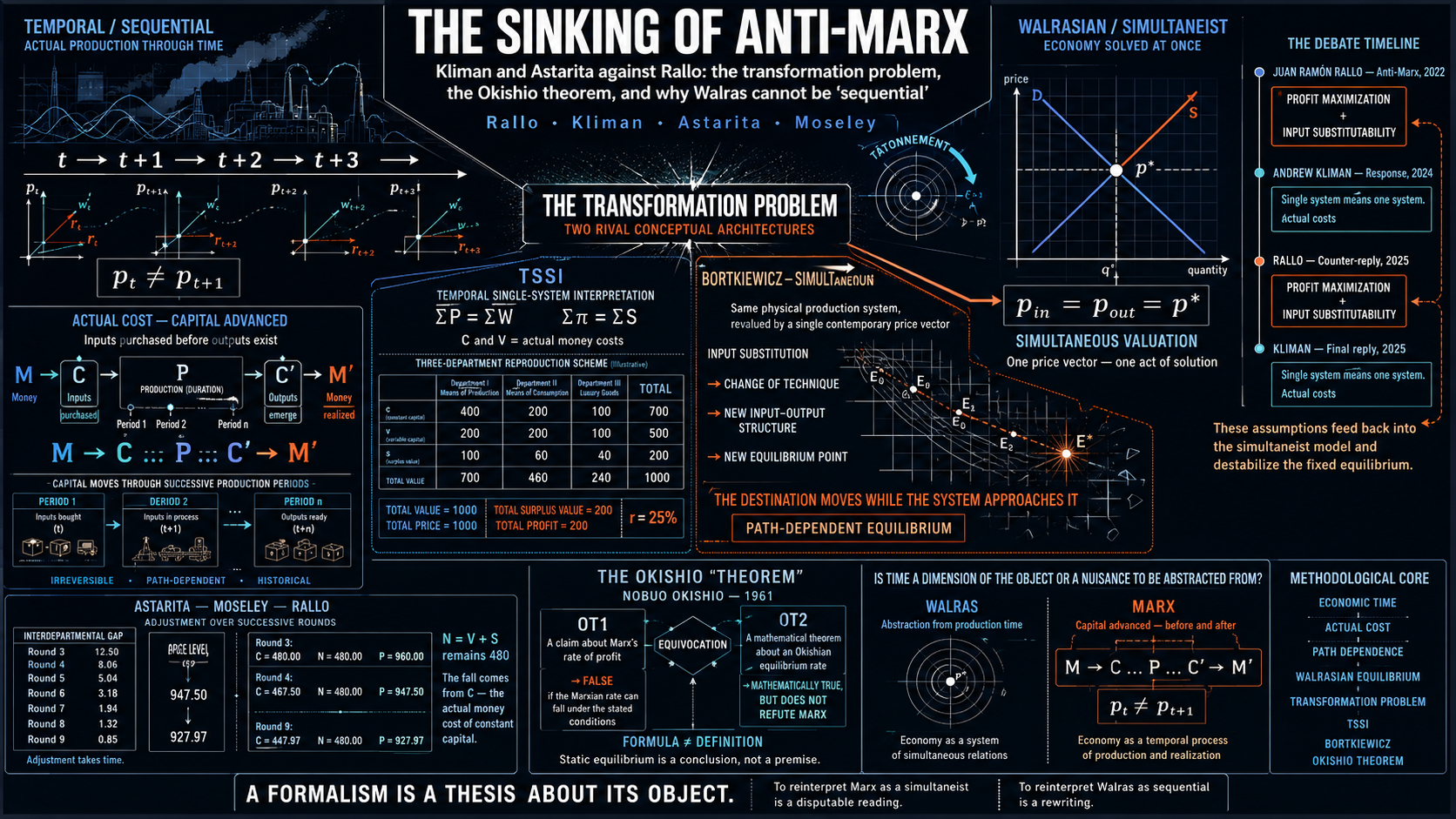
    For over a century, a single mathematical argument has been wielded as the definitive proof that Karl Marx’s economics doesn’t work. It goes like this: Marx claimed that the value of goods is determined by the labor that produces them, and that market prices eventually gravitate toward “prices of production” — modified versions of those labor values, adjusted for how capital-intensive each industry is. But when you try to verify this with a system of simultaneous equations, the numbers don’t add up. The sums of values don’t equal the sums of prices. The theory, critics have said since the early 1900s, contains a fatal algebraic error.

    This paper — spanning 260 pages and drawing on philosophy, history, sociology, and statistics — argues that the error was never Marx’s. It was the error of the people who checked his math using a method he never used.

    The Photograph vs. the Movie

    Imagine you’re trying to understand a river. You could take a photograph of it — capturing one frozen moment — or you could film it as a movie, watching how the water flows over time. For over a hundred years, the economists who criticized Marx took a photograph of his theory and then complained that it didn’t look like a movie.

    Here’s the specific issue. Marx described a two-step process: first, a general rate of profit forms across the entire economy; then, each industry’s price deviates from its pure labor value according to how much capital it ties up relative to the average. The standard critique — originating with Ladislaus von Bortkiewicz in 1907 and repeated ever since — takes all of Marx’s accounting identities and solves them simultaneously, as if input prices and output prices were determined at the same instant. Under that framework, Marx’s three aggregate equalities cannot all hold at once.

    The “inconsistency” that has been attributed to Marx for over a century is the inconsistency of the simultaneous-dualist framework that was imposed on him, and it dissolves as soon as time is restored. — Gómez Julián, summarizing the central thesis

    But here’s the catch: solving everything simultaneously is equivalent to assuming that the economy is a photograph — that there is no time. And Marx’s entire framework is built on the opposite premise: that the economy is a process, an unfolding sequence in which the prices that exit one period become the input prices that enter the next. Once you restore that temporal dimension, the “inconsistency” vanishes. The three equalities hold simultaneously — not because Marx was secretly consistent in some miraculous way, but because the contradiction was an artifact of the framework imposed on him, not of his own logic.

    The paper calls the simultaneous approach “Walrasian Marxism” — a phrase that captures the irony: economists imported the logic of Léon Walras’s general equilibrium theory and used it to read Marx, then blamed Marx when the result didn’t work.

    In Plain Language

    Marx was accused for over a century of getting the arithmetic wrong. What actually happened is that someone redid his arithmetic under an assumption he never made — that the prices of things you buy to produce and the prices of things that come out of production are the same prices, set at the same time. If you assume that, Marx’s accounts don’t close. But that assumption is equivalent to saying the economy doesn’t happen in time.

    But Was the Movie Real?

    Pointing out that Marx’s logic works when you read it correctly is necessary but not sufficient. The “temporalist” school has been making this argument for nearly fifty years. But the author noticed a critical gap: nobody in that school had ever taken real-world data and actually estimated the three types of prices Marx described — direct labor values, prices of production, and market prices — and then tested whether market prices actually gravitate toward prices of production as the theory predicts.

    This matters because, as the paper puts it, leaving the correct reading of Marx “in the territory of conceptual argumentation while the incorrect reading occupies alone the territory of measurement” is a strategic vulnerability. If you can’t show that real prices behave the way your theory says they should, your theory remains a philosophical argument, however internally consistent.

    But before presenting any numbers, the paper devotes substantial space to establishing that the process Marx described actually happened in history. This is not an appendix; it’s a foundational part of the argument.

    Before Capitalism

    In pre-capitalist societies, exchange was regulated by labor time — not because someone enforced a theory, but because the material conditions made it so. Barter was dominant, inflation did not exist, and prices could only reflect production costs given available technology. Evidence from anthropology (Malinowski’s Trobriand Islands studies), sociology (Mauss on gift exchange), accounting history (Kula’s analysis of feudal estate records), and even paleogenomics all converge: objects were valued in proportion to the labor they embodied.

    The Transition

    The dissolution of feudal relations, the monetization of exchange, and the destruction of pre-industrial normative frameworks created the conditions for capital to move freely between industries. Thompson’s work on the “moral economy” documents how the new free-market ideology had to be violently imposed, destroying customary protections and creating an unprecedented relationship of exploitation.

    Capitalism Established

    Once barriers to capital movement were destroyed, capital flowed from commerce to industry chasing higher profits, and generalized competition forced a redistribution of total surplus value across sectors. The crisis of 1873 — which destroyed nearly half the blast furnaces in major iron-producing countries — is presented as concrete evidence of the mechanism: firms whose costs were still based on older, individually more labor-intensive methods went bankrupt when they couldn’t compete with prices of production dictated by modern technology.

    In Plain Language

    Prices of production didn’t appear the day someone wrote an equation. They appeared the day capital could freely move from one industry to another chasing the highest profit — which didn’t happen until legal, moral, and political barriers were destroyed. Before that, things were exchanged roughly according to the labor they cost, and there is more than enough evidence — ethnographic, accounting, archaeological, and genetic — to show it.

    What Is a Production Price, Exactly?

    This is where the paper moves into its most technically original territory. The author carefully separates two things that must not be confused:

    What a production price is (the explanandum): it is the expected value, over the distribution of economic perturbations, of the long-run time average of market prices. In plain language: it’s the center of gravity around which actual market prices keep spinning. Not the price they arrive at and stay at (that would be equilibrium), but the average around which they never stop oscillating.

    Key Concept

    The production price is neither an eternal, timeless equilibrium (the error of the simultaneous approach and of Walrasian economics, which takes the law as such for the whole and eliminates time) nor a chaos of prices without law (the error of empiricism, which stays at the level of individual prices and loses the law). It is the law of the whole realizing itself through the contingency of the parts.

    How each step of the process works (the explanans): a rule that determines this year’s market price from last year’s market price and last year’s latent production price, and nothing else. This is modeled as a hierarchical Ornstein-Uhlenbeck process — a three-level cascade in which the production price is itself a latent state with its own dynamic gravitating toward value, and market prices gravitate toward that latent state rather than toward a fixed, noisy index.

    The uncertainty is built into the model explicitly: uncertainty in the average rate of profit, uncertainty in the advanced capital, uncertainty in the disaggregation of national accounts into 37 sectors (handled through multiple imputation with 25 imputations combined by Rubin’s rule), and parametric uncertainty estimated through Bayesian Markov Chain Monte Carlo methods.

    One crucial point: no magnitude is obtained by solving a simultaneous system. Value is constructed empirically and directly as $V = c + v + p$ (cost plus surplus value), and production price as $\Phi = c + K \cdot G’$ (cost plus capital times the general rate of profit). There is no Leontief inversion, no simultaneous algebra, anywhere in the construction.

    In Plain Language

    Think of a production price as the “gravitational center” of a spinning object. The object (a market price) never stops moving — it wobbles, it swings, it drifts — but over time its average position is pulled toward that center. The math describes both what the center is and how each wobble happens, and it does so while honestly accounting for all the uncertainty in the measurement.

    The Defining Equations: (9) Through (11)

    Here is where the metaphor turns into mathematics. The paper writes the definition of a production price in three successive steps — each one making explicit an assumption the previous step left implicit — numbered (9), (10), and (11) in the original text. None of the three generates a trajectory by itself; together they define the explanandum — what the object is — that the cascade below then generates.

    Equation 9 — What a Production Price Is
    $$ \lim_{t\to\infty} E\!\left[\varphi^i_t\right] \;=\; k^i_t + K^i_t\, E\!\left[G'(t,X)\right] \;=\; \Phi^i_t $$

    Here $\varphi^i_t$ is sector i’s market price at time $t$, $k^i_t$ is its cost price (constant capital consumed plus variable capital), $K^i_t$ is the total capital advanced, and $G'(t,X)$ is the general rate of profit — itself a stochastic process indexed by a perturbation $X$ that bundles the exodus of capital between branches and technological innovation.

    In words: a production price is the long-run limit of the average market price. Not the price itself at any instant — that keeps oscillating forever — but where its time-average settles as the horizon stretches out. Notice the object on the right-hand side, $k + K \cdot E[G’]$: it is the same accounting identity introduced earlier (cost price plus the average profit rate applied to capital advanced), except the profit rate is now written as an expectation, because it fluctuates.

    Equation 10 — Making the Averaging Explicit
    $$ \Phi^i_t = \lim_{t\to\infty} E\!\left[\varphi^i_t\right] = \int_{-\infty}^{\infty} \!\left(\lim_{t\to\infty} \varphi^i_t(x)\right) f_X(x)\, dx \;=\; k^i_t + K^i_t \int_{-\infty}^{\infty} G'(t,x)\, f_X(x)\, dx $$

    $f_X$ is the probability density of $X$. The equation says the expectation is an average over every possible state $x$ of the system’s turbulence, weighted by how likely that state is.

    Equation (10) earns its keep by making a subtle move legitimate: swapping the order of the limit and the expectation. That looks harmless, but it hides a real question — does the market price $\varphi^i_t$ even converge to anything as $t \to \infty$? The paper’s answer is no: a capitalist system doesn’t settle into a fixed point, it settles into a limit cycle — perpetual oscillation. So the convergence the argument needs isn’t of the instantaneous price, but of its cumulative time-average. That average does converge, for almost every state of the world, precisely because the system is ergodic — the fraction of time the cycle spends in each region of its orbit stabilizes. This is the Birkhoff ergodic theorem doing, in mathematical language, exactly what Marx says in economic language: the production price isn’t the value the market price reaches and stays at, it is the average around which it never stops oscillating. The oscillation isn’t an obstacle to the average — it is the average’s condition of existence.

    Why the Order of Operations Matters

    The paper invokes Lebesgue’s Dominated Convergence Theorem to justify swapping “limit of the average” for “average of the limit.” This requires bounding market prices by some integrable envelope — economically, that no price can grow without limit, which technological ceilings and competitive pressure guarantee — and, crucially, it does not require that the convergence be uniform across sectors. Uniform convergence would mean competition equalizes profits instantly and identically everywhere, with no room for a shock to hit one industry harder than another. Marx’s theory says the opposite, and the math is built to allow it.

    Equation 11 — When the Capital Base Is Also Uncertain
    $$ \Phi^i_t = \lim_{t\to\infty} E\!\left[\varphi^i_t\right] = \int_{-\infty}^{\infty}\!\!\int_{-\infty}^{\infty} \left[k^i_t + K^i_t(y)\, G'(t,x)\right] f_{X\mid Y}(x\mid y)\, f_Y(y)\; dx\, dy $$

    Equation (10) still treated the capital base $K^i_t$ as known exactly. Equation (11) drops that simplification: $Y$ is a second random variable carrying the estimation error in $K$, with density $f_Y$, and $f_{X \mid Y}$ lets the profit-rate perturbation depend on which realization of that error occurred. The object is the same double average — only now uncertainty is propagated from two sources instead of one.

    This last equation is not a mathematical flourish; it is the reason the empirical section spends so much effort on multiple imputation. National accounts don’t hand anyone a clean measurement of capital advanced by sector — it has to be reconstructed from incomplete data, and that reconstruction carries its own error. Equation (11) is the license to treat that error as a random variable to be averaged over rather than a nuisance to be ignored. The uncertainty is propagated externally — by a generator outside the statistical model itself — rather than estimated as an internal parameter of the dynamic model: estimating $K$’s error inside the model would confound it with the model’s own measurement-noise term, opening a ridge of non-identification between two magnitudes that the data alone cannot tell apart. Kept external, twenty-five complete reconstructions of the data are generated first, each respecting the Marxian aggregate identities to machine precision, the dynamic model is fit on each, and the twenty-five fits are combined by Rubin’s rule. That is the outer average of equation (11), computed by literally drawing from the distribution of $Y$ instead of assuming it away.

    The Engine: A Three-Level Ornstein–Uhlenbeck Cascade

    Equations (9)–(11) define the target; they don’t generate a path toward it. The explanans — the mechanism that actually produces a year-by-year trajectory consistent with that target — is a hierarchical Ornstein-Uhlenbeck process with up to three nested levels, fit as a single Stan program (the same program handles one, two, or three levels, which guarantees that adding levels can never silently break the simpler cases nested inside them). All series enter standardized; time is discretized one year at a time using the Euler–Maruyama scheme.

    Level 1 — The Market Price
    $$ dev_{t,s} = \varphi_{t-1,s} – \Phi_{t-1,s} $$
    $$ \kappa^m_{t,s} = \kappa_{\mathrm{cap}} \cdot \mathrm{invlogit}\!\left(\kappa_s + \beta_1\, z^{TMG}_t\right) $$
    $$ \Delta\varphi_{t,s} = \kappa^m_{t,s}\!\left(-\,dev_{t,s}\right) \;+\; a_{3,s}\, dev_{t,s}^{\,3} \;+\; \gamma\, COM^{std}_{t,s} \;+\; \varepsilon_{t,s} $$

    Subscripts $s$ (sector) and $t$ (year) run throughout. $dev$ is last year’s gap between market price and the latent production price. $\kappa^m$ is the sector’s reversion speed, passed through a logit link that caps it inside $(0, \kappa_{\mathrm{cap}})$ and lets the general rate of profit ($z^{TMG}$) modulate it without ever pushing the system out of the stable region of the discretization. $\varepsilon$ is a fat-tailed (Student-t), stochastic-volatility innovation, so volatility can cluster in time without destabilizing the mean.

    Read the Level 1 line as a spring. The term $-\kappa \cdot dev$ is the restoring force: it pulls the market price back toward the production price with a force proportional to how far it has drifted. The cubic term $a_{3,s} \cdot dev^3$, with $a_{3,s}$ constrained negative by construction — not estimated, imposed — makes that restoring force grow faster than proportionally once the deviation gets large: the further the market strays, the harder it snaps back. This is a declared stability assumption, not a discovery: it guarantees the model can never generate an explosive regime, at the real cost that if such a regime existed in some sector of the actual economy, this particular specification could not detect it.

    Levels 2–3 — Where the Latent Center Itself Reverts
    $$ \mu_{s,t} = m_{0,s} + m_1\, G’_t + m_v\, V_{s,t} $$

    The production price $\Phi$ is not treated as a fixed, observed index; it is itself a latent state that reverts — more slowly, with its own sector speed $\kappa_p$ — toward this mean $\mu$. $m_1$ is the channel running through the general rate of profit; $m_v$ is the coefficient measuring how strongly the production price tracks the directly-constructed value $V_{s,t} = k + p$ (Level 3, and the reason the cascade goes up to three levels rather than stopping at two).

    This is the bridge back to the abstract equations above, term by term. $\mu_{s,t}$ is the estimable stand-in for the right-hand side of (9): $m_{0,s} + m_1 G’_t$ plays the role of $k + K \cdot E[G’]$, and $m_v V_{s,t}$ is the specific functional form chosen for the value-tracking channel that the abstract definition deliberately leaves open (the paper is careful to say that capitalist competition as a function of the value structure is declared at the level of equations 9–11, not derived; giving it the concrete shape $m_v V$ is a modeling choice made at the cascade level, defended by how it performs under validation rather than deduced from the definition). And the expectation of $G’$ from equation (9) has its operational counterpart in the profit rate averaged across the twenty-five multiple imputations — the mechanism equation (11) licenses.

    The coefficient $m_v$ carries real theoretical weight: it is the empirical stand-in for Chapter 9’s claim that prices of production gravitate around values. It is given a neutral prior, $m_v \sim \mathcal{N}(0,\, 0.5)$ — centered at zero, symmetric, assigning equal plausibility to $m_v > 0$ and $m_v < 0$ before seeing any data. That matters for the same reason a fair coin matters in a coin-flip experiment: if the data carried no signal, the posterior would sit wherever the prior put it, hugging zero. It doesn’t. It lands at $m_v \approx 1.0136$ with $P(m_v > 0) = 1$ — evidence that the data moved it there, not the prior. The anchoring to value is found, not assumed into the setup.

    In Plain Language

    The cascade is three springs stacked on top of each other. The market price is tied by a spring to the latent, unobserved production price. The production price is tied by its own, slower spring to a moving target that blends the general rate of profit with the directly-measured labor value. Pull any one spring and let go: it doesn’t snap to a fixed point, it settles into the kind of perpetual, decaying oscillation that equations (9)–(11) describe as an average. The springs are estimated from sixty-one years of real U.S. data, not assumed; the coefficient tying prices of production to values, specifically, could have come back negative or zero — the model gave it every chance to — and it didn’t.

    What the Numbers Say

    The empirical core of the paper is a panel of 37 productive branches of the United States economy over 61 years, from 1960 to 2020. The hypothesis tested encloses three distinct relationships, and the paper is meticulous about not conflating them. Each is stated, tested, and reported separately.

    Market Prices ↔ Prices of Production: The Strongest Link

    This is the relationship with the firmest statistical support, confirmed through six independent lines of evidence:

    Central Finding

    Gravitation exists, and it is slow. The median speed across sectors is $\kappa_m = 0.0770$, equivalent to a half-life of approximately 9 years. Market prices take about a decade to cover half the distance toward their production-price center. This is consistent with Marx’s characterization of gravitation as a tendential, mediated regulation, not an instantaneous fit.

    The number is remarkably stable under stress tests:

    • Removing five of the six productive blocks from the panel barely moves the estimate — it shifts in the third decimal place. The sixth, which gathers 18 of the 37 sectors, does produce a shift (from 9 years to 6 years), and the paper decomposes it: about half the acceleration is the generic effect of halving the panel — removing 18 sectors at random already gives 0.0929 — and not the block itself.
    • Dismantling the value anchor in three different ways — including permuting surplus value across spheres — moves the speed in the third decimal place. This is significant: it means the conclusion about market-to-production gravitation does not depend on the less robust production-to-value link.
    • The market deviation has its own dynamic signature. Compared against a random walk matched in variance, three out of six test statistics separate cleanly (the weighted-sum convergence reaches a tolerance of 0.01 while the null never reaches a tolerance ten times more lenient; recurrence analysis laminarity triples the null; recurrence entropy doubles it). The ones that don’t separate are recurrence-analysis determinism and the two deterministic-chaos invariants — the Lyapunov exponent and the correlation dimension — which the paper never claimed to find.
    • The estimate is invariant to secondary methodological choices. Sweeping the latency regularizer across three values produces life medias of 9 years in all three arms (speeds of 0.0774, 0.0770, 0.0772).
    • The known bias of disaggregation pushes against the result. Splitting a national figure among 37 branches is underdetermined and biases speed estimates downward — meaning the true half-life is probably 7–8 years rather than 9. A bias that works against your conclusion is one you can live with, because the result holds despite it, not thanks to it.

    Prices of Production ↔ Values: The Thinnest Leg

    This is the weakest part of the empirical argument, and the paper states so with complete transparency. The problem is not a defect of the instrument but a property of the object:

    Methodological Transparency

    The coupling coefficient estimated within the dynamic model is $m_v = 1.0136$ with a 95% credible interval of $[1.0096,\; 1.0176]$ — but the same procedure returns 1.0365 when surplus value is permuted across spheres, preserving all annual aggregates. Why? Because production price and value share the cost price, which explains 66.1% of the variance of the former and 72.0% of the latter, and their correlation in levels is 0.9987. The coefficient would land near one even if the law of value didn’t hold at all. The paper therefore reports it as a consistency check, not as evidence.

    The real support for this relationship comes from cross-sectional tests, not from the dynamic coupling. When temporal common trends are removed and analysis is conducted within-year, the slope of the markup on own surplus value is 0.675 with the true data versus 0.090 under permutation, with intervals that don’t come close to overlapping. The sectoral ordering of the wedge between $\Phi$ and $V$ has an inter-annual rank correlation of 0.986 and a 60-year value of 0.558 — highly persistent structure, not noise.

    A collateral finding worth noting: the coefficient of variation of sectoral profit rates is 0.669 — meaning profit rates across industries show considerable and persistent dispersion. Far from contradicting the theory, this dispersion is the condition of existence of the mechanism: if profit rates were already equalized, there would be no differential to drive capital migration, and gravitation would have nothing to operate on. Marx postulates equalization as a tendency, not an accomplished fact.

    Market Prices ↔ Values: Sustained in Form, Adjusted in Existence

    The structural modification across sectors exists and is nonlinear (the nonlinearity step holds comfortably at 6.8 null deviations). But the existence step is adjusted: 44% of its gain is obtained equally with sectoral characteristics unpaired from their spheres, and the gap against the maximum null is on the order of one paired standard error. The coefficients survive a deliberately severe correction for serial dependence (tripling the error).

    The Instrument Behind That Number: A Nested Ladder in gdpar

    That test is a small ladder of nested distributional-regression models, fit with gdpar (Gómez Julián, 2026b), the author’s own R package for generalized distributional parameter regression, published on CRAN on July 15, 2026. The ladder climbs from a bare model — “the market-to-value ratio has no sector-specific correction at all” — through a model where organic composition, wage share, and sector size shift that ratio linearly, up to a model where the correction is a flexible spline rather than a straight line. Two gains matter, measured in units of predictive density: adding the linear correction buys 207.3 units; letting it curve buys another 215.1. Both were checked against a control built to be hard to pass — shuffling which sector gets which characteristics 99 times, refitting each time, with the spline’s knots held fixed across every shuffle so the comparison can’t be won by a better basis alone. The curvature gain clears its null with room to spare (6.8 null standard deviations; the best of 99 shuffles reaches only 114.8 against 215.1 observed). The existence gain is honestly reported as thinner: shuffled sectors still buy about 44% of the real gain merely by having some characteristics to fit — three covariates and an intercept give a model room to accommodate noise even when it is being told nothing true — so the genuine margin over the null sits at about one paired standard error (23.2, against a gap of roughly 24 units). Both numbers are reported together, precisely so the large one isn’t read alone.

    A companion specification, estimated in the same gdpar fit, asks the same question about dispersion rather than location: not where the market-to-value ratio is centered, but how tightly it clusters. Larger sectors and sectors with higher capital composition show systematically less relative dispersion — elasticities of $-0.226$ and $-0.104$ — consistent with equalization operating more effectively where capital is more concentrated. Both effects clear a “breaking factor” (the multiple of the standard error at which the 95% interval would first touch zero) north of six and four respectively, past the 2.94 ceiling reached anywhere else among this paper’s location coefficients, and the finding reproduces under a completely different likelihood family (a gamma distribution on the price ratio) to within 5.2%.

    Three Failures That Confirm the Theory

    One of the most intellectually striking features of this paper is how it handles results that, at first glance, look bad for its thesis. There are three, and the paper reports all of them without softening — then shows deductively why each one was expected if the theory is correct.

    Negative Result No. 1

    The model does not out-of-sample predict better than a random walk. But this was deductively implied by the slow form of the thesis. At a horizon much shorter than the half-life, a mean-reverting process is, to first order, a random walk. If something takes a decade to get halfway back, looking at a single year won’t let you see it return.

    Negative Result No. 2

    The value term is predictively indistinguishable. Again, this follows from the slow coupling between prices of production and values: with half-lives on the order of decades and only 61 years of data, univariate root-unit tests are structurally underpowered.

    Negative Result No. 3

    No univariate test separates the true wedge from its permuted placebos. But this was predicted before measuring, by the persistence of sectoral ordering itself (inter-annual rank correlation of 0.986). A highly persistent time series is hard to distinguish from its permuted version using tests designed for shorter memory.

    Finding these signatures is corroboration of the slow form of the thesis, and not finding them would have been the real problem. — Gómez Julián, on the negative results

    The paper’s stance on this is worth highlighting: “Lejos de refutar la tesis, los tres están deductivamente implicados por su forma lenta” — far from refuting the thesis, all three are deductively implied by its slow form. A single mechanism (slow gravitation) explains both the substantive thesis and all the apparently negative results, and it also survives in the validated posterior. “That a single cause explains the thesis and all the apparently negative results, and that it additionally survives in the validated register, is the opposite of a petitio principii: it is a unified, falsifiable, and internally validated narrative.”

    Temporalism Isn’t a Preference — It’s a Condition of Measurement

    Perhaps the most consequential result in the entire paper is not a number but a statement about what can and cannot be measured. It concerns the “modulator” — the component of Marx’s argument in which the general rate of profit enters into the structural modification of each sphere, meaning the deviation of each sphere is not independent of the reference but generated by it.

    The Identifiability Argument

    When the model was run with a single, fixed general rate of profit for all 61 years (as a simultaneous approach would require), the posterior exhibited a flat ridge: two completely different functional bases (a degree-two polynomial and a spline basis) produced the same pathology to the third decimal place, with an effective sample size of only six draws. The diagnostic got worse with more sampling (R-hat rising from 1.33 to 1.73). This is the unmistakable signature of a direction in parameter space along which the likelihood does not change.

    The cause is theoretical, not computational. With one fixed reference, the modulator can only be identified evaluated at that single point — a single number, not a function over the space of references. You cannot estimate three coefficients from a polynomial if you have one data point.

    When the reference was allowed to vary year by year (61 different general rates of profit), the model converged within minutes, with a large improvement in both time and effective sample size, and zero divergences.

    Named, Not Improvised: Theorems 1A and 1E

    This diagnosis isn’t an ad hoc read of a misbehaving sampler. gdpar (Gómez Julián, 2026b) — the same package behind the nested ladder above — ships a formal identifiability result for exactly this situation. Its Theorem 1A establishes that, with a single fixed reference point, a distributional modulator is identified only at that point: as one number, not as a function over the space of possible references. Theorem 1E is the positive counterpart: letting the reference vary restores identifiability of the modulator as a function. Fitting a degree-two polynomial (three coefficients) or a five-knot spline basis (five coefficients) against one single, unmoving reference asks for more than a single data point in that dimension can support — which is exactly what a flat likelihood ridge looks like from the sampler’s side.

    The figures behind the improvement, precisely: a fixed reference with a degree-two polynomial gives an R-hat of 1.7333, an effective sample size of 6, and 8 divergent transitions in 39 minutes; a one-knot spline basis reproduces the same pathology — R-hat 1.7335, effective sample size 6, 14 divergences, 5.6 hours. Letting the reference vary year by year (61 distinct annual values of the general rate of profit), centering the additive component and raising the sampler’s adaptation parameter to 0.99, gives an R-hat of 1.0035, an effective sample size of 1332, and zero divergent transitions — in 2.9 minutes. That is the 115-fold improvement in time and 222-fold improvement in effective sample size referenced above, and it is a theorem, not a tuning trick: no amount of additional sampling closes that gap under a fixed reference, because the object being asked for — the modulator as a function — simply is not there to find.

    The consequence is stated precisely: with a single fixed general rate of profit obtained by solving the system simultaneously, the claim of Chapter 9 of Volume Three of Capital is unverifiable by construction. It is not that the data are insufficient — the object is not identified, and no amount of data would identify it. The argument does not establish that simultaneism is false as a description of capitalism (that is established by historiography and sociology); it establishes that a simultaneous procedure cannot, even in principle, empirically verify the specific part of Marx’s argument that this work estimates.

    In Plain Language

    Marx says: first a general rate of profit forms, then each industry deviates from it according to how capital-intensive it is. To check whether the deviation depends on the general rate, you need to see what happens to the deviation when the general rate changes. If you calculate one general rate for the entire 61-year span, it never changes, and there is nothing to observe. That is exactly what happened: the model with one fixed rate doesn’t converge — not because of computational limitations, but because it is being asked to measure a relationship with a single observation of one of the two variables. Calculating one rate per year — which is what the temporal reading says you should do — the same model converges in three minutes.

    What This Is, and What It Isn’t

    The paper is careful, almost painstakingly so, about the limits of what it claims. This section matters because a reader coming from the “pro-Marx” or “anti-Marx” side might be tempted to over-read the results. The author doesn’t let you.

    What the evidence authorizes: In the United States between 1960 and 2020, market prices gravitate toward prices of production with a decadal half-life that is sectorially heterogeneous, and this speed survives three independent assaults (removing five of the six productive blocks, destroying the value anchor, varying secondary methodological decisions). This is a measured, calibrated, and falsifiable fact.

    What the evidence does not authorize:

    • It does not claim superior predictive power (the model does not out-predict a random walk, which was expected).
    • It does not claim that univariate root-unit tests confirm gravitation (they are structurally underpowered at this time scale).
    • It does not claim uniqueness or categorical novelty. The contribution is the explicit integration and canonization of a slow gravitation cascade with value anchoring, measured on real data, with propagated uncertainty, validated, and subjected to a diagnostic whose unfavorable results are reported alongside the favorable ones.
    • It does not claim that this statistically demonstrates the law of value, “and not for rhetorical prudence but because it would be false: a price series can show that a magnitude behaves as the law predicts, and cannot explain why that magnitude exists or whether the category with which we name it is the correct one.”

    That last point is the paper’s deepest epistemological commitment. Questions about whether “value” is the right category for what prices ultimately measure are not answerable by any price series, no matter how long. They are answered by history, sociology, and philosophy — and the firm answer is the one obtained when all four disciplines (those three plus statistics) point in the same direction. The four-dimensional convergence is the argument, not any single leg of it.

    The paper also addresses the homology that unifies its seemingly disparate halves — the historiographical-filosofical first chapter and the econometric second chapter. The relationship between necessity and contingency that governs the transition from feudalism to capitalism (where the same demographic shock produced opposite outcomes in different regions of Europe) is structurally identical to the relationship between prices of production and market prices. A law determines the center; circumstances determine each particular outcome. Neither fact negates the other, because they describe different levels of the same reality.

    What It All Adds Up To

    Here is the simplest version of what this 260-page paper establishes:

    Marx was reproached for a century for having done an arithmetic calculation wrong. What happened is that his calculation was redone under an assumption he never made: that the prices of things bought to produce and the prices of things that come out of production are the same prices, fixed at the same time. If you assume that, Marx’s accounts indeed don’t close. But that assumption is equivalent to saying the economy doesn’t happen in time. As soon as you accept that what exits the factory this year is what enters the factory next year, the accounts close without anyone having to fix anything. — Gómez Julián, Summary for the Reader

    But recognizing the conceptual error was only the first half. What had been missing — and what this paper contributes — is doing those accounts with real data instead of with fictitious numerical examples, which is what the school that had the correct conceptual reading had never done.

    The empirical results show that prices in the U.S. economy over six decades do behave as the theory predicts: they gravitate, slowly, toward prices of production calculated with Marx’s theory and no other. This finding survived every attack the author could devise — removing productive sectors, destroying the value anchor, permuting surplus values, varying methodological decisions, and running diagnostics whose unfavorable results are reported in full alongside the favorable ones.

    The part of the argument linking prices of production to labor values is also supported by real evidence, though less firmly, and the paper says exactly where the weak points are and why they are properties of the object, not defects of the instrument.

    And the paper does not claim to have demonstrated the law of value with a series of numbers, because “questions of that kind are not answered with numbers: they are answered with history, with sociology, and with philosophy, and the firm answer is the one obtained when the four things (the previous three, together with statistics) all point in the same place.”

    That convergence doesn’t make the result eternal — better evidence can overturn it tomorrow. But it makes it, for now, “our best possible approximation to the truth.”

    — — —

    “In science as in life, overcoming adversity is what makes us truly strong.”

    This post summarizes the introduction, conclusions, and the formal-empirical chapter (§2.4) of Gómez Julián, J. M. (2026). Some Reflections on Marx’s Prices of Production: Historicity of the Law of Value, Dialectical-Materialist Foundation, and Dynamic Formalization Under Uncertainty. Zenodo. https://doi.org/10.5281/zenodo.21842251. The full paper spans approximately 260 pages across two chapters covering philosophy, historiography, mathematical formalization, and empirical econometrics. Equations (9)–(11) and the model specification cited here reproduce that chapter’s notation; gdpar is cited separately as Gómez Julián (2026b).

    Written for the curious. An invitation to read.

  • Is It Scientifically Possible for Central America To Be a Single Country?

    Is It Scientifically Possible for Central America To Be a Single Country?

    Political Science & History

    Science, Youth, and the Rebirth of a Central American Nation

    The Origins of Scientific Unionism in Central America and Its Unavoidable Future

    History is rarely kind to fragmented nations. At the dawn of the 20th century, Central America was a collection of small, vulnerable republics plagued by authoritarian rule, economic volatility, and the looming shadow of international imperialism. Yet, from the cloistered halls of the University of San Carlos in Guatemala, a quiet revolution was brewing. It was led not by generals, but by students. This is the story of how a group of young intellectuals pioneered “Scientific Unionism”—a movement to reunite Central America not through romantic nostalgia, but through the rigorous application of social sciences.

    Based on Margarita Silva Hernández’s illuminating research, this post explores the historical genesis of this movement. Furthermore, it asks a vital question for today’s political scientists and economists: If Scientific Unionism was valid a century ago, is it not an absolute, long-term historical inevitability for Central America’s survival on the global stage today?

    The Catalyst: 1898 and the Shift in Global Power

    To understand the birth of Scientific Unionism, we must look at the pivotal year of 1898. The Spanish-American War resulted in a resounding victory for the United States, establishing it as a first-rank global power with expansionist ambitions in the Caribbean and Central America. For a group of young university students, this was not merely a geopolitical shift; it was an existential threat. They perceived the conflict as a clash between the Anglo-Saxon and Latin worlds, sparking a profound anti-imperialist consciousness.

    Simultaneously, the region was suffering the aftershocks of the 1897 coffee price crash. The liberal economic model, heavily reliant on agricultural exports and foreign capital (like the newly formed United Fruit Company), had left the isthmus vulnerable. The students saw the economic crisis as a symptom of a deeper disease: the fragmentation of Central America. To them, the petty dictators of the region were complicit in this backwardness, suppressing social mobility and selling out national resources.

    The Birth of Scientific Unionism

    On June 18, 1899, a clandestine group of students formed a society called El Derecho (The Law). Led by a young Nicaraguan, Salvador Mendieta, these students—mostly in their late teens and early twenties—originated from across the isthmus. They were the children of provincial merchants and professionals, united by a shared frustration with the lack of political mobility under authoritarian regimes.

    What set El Derecho apart from previous attempts at Central American unity was their methodological approach. They did not want to simply restore the old Federal Republic of the 1820s through military decrees. Instead, they turned to sociology. Influenced by the positivist ideas of Auguste Comte, Herbert Spencer, and John Stuart Mill, they sought to discover the “social laws” governing Central America.

    “They designated their movement ‘scientific unionism’ to evidence the intellectual condition of its founders and the scientific-social bases of their working methods.”

    Their thesis was clear: Central America was a single nation artificially divided. To reunite it, one could not rely on mere political pacts (which had repeatedly failed, such as the brief “Greater Republic” in 1898). Instead, they needed to build a cultural unity. They believed that through civic education, the eradication of localism, and the application of scientific principles to governance, they could forge a strong, unified state capable of resisting foreign intervention and achieving modernization.

    From Theory to Political Action

    The students of El Derecho did not remain in the classroom. They organized five Central American Student Congresses between 1901 and 1911, creating a regional network of young thinkers. They published pamphlets, established night schools for workers, and delivered public conferences. They positioned themselves as the intellectual vanguard destined to replace the old oligarchic guard.

    Naturally, this provoked the wrath of local dictators. Manuel Estrada Cabrera in Guatemala met their denunciations with brutal repression. Students were imprisoned—some, like Marciano Castillo, dying in the penitentiary—and the movement was forced into exile. By 1904, the students had evolved into a formal political entity: the Central American Unionist Party (PUCA). The student movement had matured into a regional political force.

    A Modern Perspective: The Inevitability of Union

    The preceding sections summarize the historical findings of Margarita Silva Hernández. The following section represents the extrapolation of this blog’s author, using the historical foundation of Scientific Unionism to pose contemporary political and economic questions.

    When Salvador Mendieta and his peers looked at Central America in 1899, they applied the scientific method to diagnose a fractured region. If we apply modern political science and economic theory to Central America today, does the scientific case for union remain valid? The data suggests not only that it is valid, but that it has become a historical inevitability.

    Geopolitical Scale and Relevance: In the 19th century, Mendieta feared absorption by the US. Today, the threat is irrelevance in a multipolar world dominated by giants. A united Central America would encompass a territory of approximately 423,000 square kilometers—larger than Germany. This is not merely a trivia fact; it implies a geopolitical footprint capable of negotiating on equal terms with global powers, managing its own maritime routes, and securing a strategic position between two oceans.

    Diversifying the Production Matrix: Historically, the region has suffered from a monoculture export model (coffee then, and various agricultural or low-tier assembly maquilas now). A unified state would possess an unprecedented diversity of microclimates, resources, and cultural demographics. This diversity would allow for a scientifically planned diversification of the production matrix. The agricultural backbone (coffee, bananas, sugarcane, livestock) would not be abandoned, but rather complemented. A single Central American market of over 50 million people provides the necessary domestic consumer base to justify intense, state-sponsored industrialization. It creates a rationale for heavy infrastructure, regional supply chains, and a unified digital economy.

    The Science of Scale: Modern economics validates the original premise of Scientific Unionism. Fragmented states suffer from duplicated bureaucratic costs, border frictions, and an inability to capture economies of scale. A unified Central America would eliminate these inefficiencies. It could pool its scientific and intellectual capital—much like the students of El Derecho envisioned—into a single educational and technological ecosystem.

    Therefore, the question is no longer merely historical. If Central America wishes to be more than a peripheral zone of extraction for larger economies, union is not a romantic dream of the past; it is a scientific, economic, and historical necessity for the future. The students of 1899 understood the math of their era. We must be brave enough to do the math of ours.

    ~ Exploring the past to architect the future ~

  • BITOPOLOGICAL SPACES: LISTENING TO THE DIRECTION OF TIME WHEN IT MATTERS

    BITOPOLOGICAL SPACES: LISTENING TO THE DIRECTION OF TIME WHEN IT MATTERS

    Bitopological Spaces: Listening to the Direction of Time When It Matters

    Bitopological Spaces: Listening to the Direction of Time When It Matters

    How two topologies — built from the same data — can hear the difference between past and future

    Most of the tools we use to analyze sequences of data — averages, correlations, spectral analyses — treat time as a label that could run in either direction without changing the answer. Reverse the order of your data points and many standard methods give you identical results. But in the real world, the direction of time matters profoundly. Economies expand slowly and crash suddenly. Heartbeats rise smoothly and fall steeply. A method blind to direction is a method blind to one of the most fundamental features of how systems change.

    A recent paper by independent researcher José Mauricio Gómez Julián introduces a construction that addresses this gap. Taking a known method from graph theory and extending it to directed graphs, the paper produces a pair of topologies — mathematical frameworks for understanding structure and connectivity — whose divergence is a topological fingerprint of temporal irreversibility. Applied to three decades of American economic data, the method recovers a picture that is both mathematically precise and economically interpretable. Here is a walk through the main ideas.


    Seeing and Being Seen

    The starting point is a beautifully simple idea introduced by Lucas Lacasa and collaborators in 2008. Imagine plotting a time series — say, 129 consecutive quarterly growth rates of U.S. GDP — as points above a timeline. Now connect two points with a line if they can “see” each other: the straight segment between them passes above every intermediate data point, as if you stood at one point and shone a flashlight toward the other with no obstacles in the way.

    The result is a visibility graph: a network whose nodes are time points and whose edges encode a geometric relationship. Visibility graphs have been used to classify chaotic systems, detect heartbeat anomalies, and distinguish between types of economic regimes. They translate the shape of a time series into the structure of a graph, opening the door to the vast toolkit of network science.

    But standard visibility graphs are undirected: an edge between two points does not record which one came first. If you orient each edge from the earlier time point to the later one, you obtain a directed visibility graph — a directed acyclic graph in which the arrows always point forward in time. This orientation carries information about temporal asymmetry that the undirected graph throws away entirely.

    From Networks to Structure

    Here is where the paper’s contribution begins.

    In 2018, Huda Nada and collaborators introduced a procedure for turning any undirected graph into a topological space. For those unfamiliar with the term, a topology is a mathematical framework that defines what it means for groups of points to be “open,” for sets to be “connected,” and for spaces to have “structure.” It operates at a level more abstract than distances or coordinates — it captures the pattern of how sets overlap and separate.

    The Nada construction works as follows. For each vertex of the graph, compute its closed neighborhood: the vertex itself plus all of its immediate neighbors. Take this family of neighborhoods and generate a topology by closing it under two operations: finite intersections (combine neighborhoods by overlapping them) and arbitrary unions (combine neighborhoods by collecting them). The result is a topology on the vertex set, and its invariants — connected components, separation properties, component counts — capture structural features of the graph.

    This procedure is universal: it works for any family of subsets of any set. The mathematical content lies in identifying the right family to use.

    Gómez Julián’s key observation is that for a directed graph, you do not get one family of neighborhoods — you get two. For each vertex:

    The forward closed neighborhood includes the vertex itself and all the vertices it points to — the later time points it can see. The backward closed neighborhood includes the vertex itself and all the vertices that point to it — the earlier time points from which it is visible.

    Apply the Nada procedure to the forward neighborhoods and you get a topology τ+. Apply it to the backward neighborhoods and you get a topology τ. The resulting triple (V, τ+, τ) is what mathematicians call a bitopological space: a set equipped with two topologies simultaneously, a concept introduced by John Kelly in 1963.

    The extension is, in a precise mathematical sense, trivial — the topology axioms do not care where the generating family came from. But recognizing this trivial extension as the right thing to do, and showing that the resulting bitopological structure captures something real about temporal asymmetry, is the paper’s central insight.

    When Two Topologies Disagree

    If the process generating your data is symmetric — equally likely to go up as down, at the same speed — then the forward and backward neighborhoods are statistically exchangeable. The two topologies τ+ and τ look the same, and the bitopological structure adds nothing beyond the undirected construction.

    But if the process is asymmetric, the two topologies diverge. Consider the prototypical asymmetry of economic and physical systems: gradual expansion followed by sudden contraction. Forward visibility through a gradual rise connects many points — each point can see far ahead through the gentle slope. Backward visibility through an abrupt drop connects few — the sharp fall blocks the line of sight. The forward topology ends up more connected (fewer separate components) than the backward topology.

    This divergence is the topological fingerprint of temporal irreversibility. The paper defines three quantitative measures of it:

    The asymmetry direction Δ = C − C+, where C+ and C are the numbers of connected components in the forward and backward topologies. Positive Δ means the forward topology is more connected. The component-count irreversibility index IC, which normalizes the difference to lie between 0 and 1. And the base-size irreversibility index IB, which measures the analogous difference in the sizes of the generating bases.

    These are pure numbers — no calibration, no free parameters, no training data. They emerge from the structure of the data and the construction itself.

    If you reverse the direction of time in your data and the topologies change, something in the process that generated the data is irreversible — and the gap between the two topologies measures exactly how much.

    Peeling the Onion: Three Layers of Structure

    One of the paper’s most clarifying contributions is the identification of three nested layers of topological structure on the same time series, each revealing different information.

    Layer 1 — The Alexandrov topology (reachability). For a directed acyclic graph, the most basic topology treats as “open” any set that is closed under forward reachability: if a node is in the set, all its descendants are too. This topology has exactly one connected component for any weakly connected graph, because every node can reach every later node through some directed path. At this level, the system is globally indecomposable. It tells us what we already know: the economy is a single connected process in which each quarter influences every subsequent quarter through chains of causation.

    Layer 2 — The undirected Nada topology (local fragmentation). When you apply the Nada construction to the undirected shadow of the visibility graph, the topology fragments dramatically. The intersection closure of the neighborhoods reveals clusters of time points that share local structural similarity — groups of observations linked by overlapping visibility neighborhoods — that go beyond mere reachability. This layer uncovers genuine structure that the reachability topology hides entirely.

    Layer 3 — The bitopological layer (temporal asymmetry). When you split the construction into forward and backward, a further distinction emerges. The forward and backward topologies have different component counts — and the difference is invisible to the undirected construction and invisible to the Alexandrov construction. It lives only in the gap between the two directed topologies.

    Each layer is contained within the next: the Alexandrov topology is a subtopology of the Nada topology (a theorem proved in the paper), which in turn underlies the bitopological structure. But each coarser layer hides information that the finer layer reveals.

    What the American Economy Looks Like Through a Topological Lens

    The paper applies the full pipeline to the quarterly growth rate of U.S. real GDP from Q1 1992 to Q1 2024 — 129 observations spanning the dot-com bust, the Global Financial Crisis, and the COVID-19 shock. Two graph constructions are used: the Horizontal Visibility Graph and the Natural Visibility Graph, both in their directed forms.

    The headline finding is that Δ = +4 in both constructions. The forward topology has 4 fewer connected components than the backward topology, regardless of which visibility-graph variant you use. This positive value is consistent with the well-documented asymmetry of the American business cycle over this period: expansions are gradual and sustained (1992–2000, 2001–2007, 2009–2020), while contractions are sharp and short-lived (2001, 2008–2009, 2020). Forward visibility through a gradual expansion is unobstructed; backward visibility through an abrupt contraction is fragmentary.

    What makes this finding compelling is its invariance. The HVG and NVG produce very different graphs — 248 vs. 406 edges, different base sizes, different absolute component counts — yet they agree on the sign and magnitude of Δ. The signal appears robust: a feature of the underlying data, not an artifact of how you choose to draw the graph.

    Another detail worth noting: the base-size irreversibility index IB is exactly zero in both constructions. The forward and backward topologies are generated by bases of equal size (250 and 250 for the HVG, 239 and 239 for the NVG). The asymmetry lives entirely in the structure of those base elements and how their intersections distribute — not in how many there are. The two topologies are built from the same number of building blocks, but those blocks fit together differently depending on whether you are looking forward or backward through time.

    A Single Shock

    Perhaps the most striking empirical finding is what the topology says about the COVID-19 shock.

    The second quarter of 2020 recorded the sharpest contraction in U.S. GDP on record — an annualized rate of roughly −31%. The third quarter recorded the sharpest rebound — roughly +33%. These are the two most extreme observations in the entire 129-quarter series, opposite in sign and opposite in economic interpretation.

    A naive analysis would naturally separate them: one is the worst crash, the other the best recovery. They sit at opposite ends of the value spectrum.

    But the Nada topology classifies them together. Under both the undirected and directed topologies, under both the HVG and NVG, these two observations belong to the same connected component.

    Why? Because the topology is not a proximity measure. It does not group points by how close their values are. It groups them by the structure of their visibility neighborhoods — which other points they can see, and how those visibility patterns intersect. Despite their extreme and opposite values, the two quarters share neighborhoods that overlap substantially. The intersection closure, which drives the Nada construction, puts them in the same cluster.

    This matches the interpretation most economists give to the event: the contraction and the rebound are two phases of a single exogenous shock, driven by the same underlying cause — the pandemic and the policy response to it. The topology recovers this interpretation from the geometry of the data alone, without any economic priors built in.

    What the topology does not claim: it does not say that the two quarters are “similar” in value (they are the two most distant observations in the entire series). It says they are structurally linked — that no topological open set separates them. The construction responds to the combinatorics of visibility, not to the metric of distance.

    Certifying the Construction

    The paper takes reliability seriously at three levels.

    Machine-checked proofs. The central theorem and related core results have been formalized in Lean 4, a proof assistant, against the Mathlib mathematical library. A computer has verified that the proofs are logically correct, with no gaps or hidden assumptions. The formalization is archived alongside the paper as part of a reproducibility bundle on Zenodo.

    Polynomial-time algorithms. Every step of the construction has an explicit algorithm with proven complexity bounds. The connected components of each topology can be computed in polynomial time without enumerating the full topology, which can be exponentially large. The key trick is to work through a combinatorial proxy for the topology called the specialization preorder, using bitset operations that are highly efficient in practice.

    Honest uncertainty. A three-valued decision procedure for pairwise connectedness reports “pairwise connected,” “pairwise disconnected,” or “undecided” — the last when the computation exhausts its resource budget. Rather than guessing, the algorithm honestly reports that it has not finished the work. This is a methodological commitment as much as a technical one: a topological statement counts as established only when the computation has completed the work that establishes it.

    No free parameters. The construction has no tuning knobs. The topological invariants — component counts, base sizes, irreversibility indices — are determined entirely by the data and the definitions. There is nothing to calibrate, nothing to overfit.

    A New Lens

    The paper does not propose to replace existing methods of time series analysis. Correlation, spectral analysis, regime-switching models, and the many other tools of econometrics and statistics capture information that topology cannot see: amplitude, frequency, distributional shape. The paper is explicit about this complementarity.

    What the topological construction offers is a new lens — one that responds to the relational structure of a time series rather than its metric structure. It asks not “how big is this change?” but “what does this change connect to, and what does it disconnect from, and is the answer different depending on which direction in time you are looking?”

    For systems where temporal asymmetry is a defining feature — business cycles, climate dynamics, physiological signals, causal event sequences — this lens may reveal structure that traditional tools, by their very construction, cannot see.

    The application to U.S. GDP is a proof of concept. The construction is general: it applies to any time series that can be turned into a directed visibility graph, which is to say, any time series at all. Whether the invariants it produces are useful features for classification, prediction, or interpretation in broader contexts is an empirical question that the paper opens but does not close.

    What it does establish is this: there exists a construction that takes a time series, produces two topologies from it, and quantifies the gap between them as a measure of temporal irreversibility. The construction is mathematically sound, mechanically verified, algorithmically tractable, parameter-free, and — when applied to the American economy across three turbulent decades — gives answers that make economic sense.

    That is a foundation worth building on.

    “Bitopological Spaces from Directed Graphs: Extending the Nada Construction to Capture Temporal Irreversibility” by José Mauricio Gómez Julián is available at Zenodo (v1.0.2, April 2026). The complete research compendium — Lean 4 formalization, R package, empirical dataset, and reproducibility notebook — is archived alongside it.

  • A DIALECTICAL MATERIALIST ANALYSIS ON PATH DEPENDENCE, IRREVERSIBILITY AND TELEOLOGY IN PHYSICAL SYSTEMS

    A DIALECTICAL MATERIALIST ANALYSIS ON PATH DEPENDENCE, IRREVERSIBILITY AND TELEOLOGY IN PHYSICAL SYSTEMS

    Why Broken Eggs Don’t Unbreak — A New Physics of History, Direction, and Purpose
    Physics • Philosophy • Foundations

    Why Broken Eggs Don’t Unbreak

    A philosopher argues that history, not mechanics, is the deepest grammar of the physical world — and that matter itself pursues stability.

    Based on a paper by José Mauricio Gómez Julián ~9 min read

    Why does a broken egg never reassemble itself? Every law governing the motion of its atoms is perfectly reversible — run the film backward and nothing in the mathematics complains. And yet, in the real world, broken eggs stay broken. This gap between what our equations allow and what nature actually does has haunted physics for over a century. A new paper from the University of Costa Rica proposes an answer that is as philosophically bold as it is mathematically precise.

    The Paradox That Won’t Go Away

    In the 1870s, the Austrian physicist Josef Loschmidt challenged Ludwig Boltzmann’s statistical explanation of the second law of thermodynamics. His objection was devastatingly simple: if the equations of motion work the same forwards and backwards in time, how can entropy — disorder — only ever increase? This is Loschmidt’s paradox, and it sits at the intersection of thermodynamics, quantum mechanics, and the philosophy of science.

    Physicists have proposed many partial answers. Some invoke the statistical improbability of reversal (there are astronomically more disordered states than ordered ones). Others appeal to cosmological boundary conditions — the universe simply started in a very special, low-entropy state. More recent work, cited in this paper, turns to information theory and Landauer’s principle (the idea that erasing information has a minimum physical cost).

    But the author — José Mauricio Gómez Julián, writing from the University of Costa Rica — finds all of these solutions insufficient. His central claim is provocative: the paradox is not in nature. It is in our models. We build theories that are fundamentally ahistorical, then act surprised when the real world — which is fundamentally historical — doesn’t obey them. The problem, he argues, is not that reality misbehaves. It is that our theories refuse to remember.

    The Core Move

    Instead of asking “Why is the macroscopic world irreversible?”, the paper reframes the question entirely: “Why do we insist on building reversible models and then call irreversibility a paradox?”

    The Philosophical Engine: Dialectical Materialism

    The paper is grounded in dialectical materialism — a philosophical tradition rooted in Marx and Engels, developed further by Hegel (in its idealist form) and by Soviet physicists like Blokhintsev and Rosental. If that sounds unusual for a physics paper, the author would say: that’s exactly the point.

    Dialectical materialism holds that reality is made of matter in motion, that contradictions are not flaws in our thinking but features of the world, and that quantitative changes eventually produce qualitative leaps. It also insists on a distinction that modern physics has muddled:

    • Epistemology — what we can know and measure (our limitations as observers).
    • Ontology — what actually exists in the world, regardless of our ability to observe it.

    This distinction turns out to be the paper’s sharpest tool. When quantum mechanics says that a particle’s position is “uncertain,” the author asks: is that uncertainty a feature of reality (ontology), or a feature of our knowledge (epistemology)? His answer is nuanced and consequential. The Schrödinger equation itself is fully deterministic — give it an initial state and a Hamiltonian, and it will predict the future wave function with perfect precision. The randomness enters only when we try to measure — when the quantum system meets our macroscopic instruments.

    In other words, probability in quantum mechanics is an epistemological resource — a powerful tool for managing complexity and incomplete knowledge — not a statement that reality itself is fundamentally random. This does not mean quantum mechanics is wrong. It means that its probabilistic character tells us about us, not about the universe.

    The author is careful, however, to distinguish this from classical Laplacian determinism. Heisenberg’s uncertainty principle, he argues, is ontological — it reflects genuine structural features of reality (the complementarity between position and momentum). So the world is deterministic in a deep sense, but not in the naive clockwork sense. It is deterministic in the way a complex, path-dependent system is deterministic: constrained, structured, lawful — but too intricate for any observer to fully predict.

    When the terrain disagrees with the map, trust the terrain

    Path Dependence: History Before Time

    Here is where the paper makes its most original conceptual move. The author argues that path dependence is more fundamental than time itself.

    What does this mean? In complex systems — economies, ecosystems, living organisms — the current state depends not just on the present conditions but on the entire sequence of events that led there. An economy with the same GDP, population, and technology as another can behave very differently because its institutions, crises, and policy choices followed a different historical path. The paper claims this is not just a feature of complex systems. It is a feature of all physical reality, at every scale.

    In this framework, time is reimagined. It is not a background parameter through which things happen (as in Newtonian mechanics), nor a dimension woven into spacetime (as in relativity), but rather a structure that records material transformations — a kind of universal memory. Space and time co-emerge as the necessary fabric for matter to develop and preserve its evolutionary trajectory.

    The author traces this insight back to Hegel’s philosophy of nature (published decades before Einstein’s relativity), where place, space, and time are understood as a unity — and where motion (and therefore matter) arises from their contradiction. The passage is striking:

    Place is spatial singularity… This perishing and regenerating of space in time and of time in space… is movement. This becoming… is the immediate, identical and existing unity of space and time: it is matter.
    — Hegel, Encyclopaedia of the Philosophical Sciences

    If path dependence is fundamental, then irreversibility is not something to be explained — it is something to be assumed, just as mathematicians assume the existence of natural numbers rather than proving it. Every broken egg, every aging star, every evolved species is evidence that the universe remembers its own history.

    A New Equation for a Remembering Universe

    The author doesn’t stop at philosophy. He proposes a concrete mathematical reformulation of the Schrödinger equation — the foundational equation of quantum mechanics — to make path dependence explicit.

    Standard quantum mechanics writes:

    Standard Form

    iℏ ∂ψ/∂t = Ĥ ψ

    where the Hamiltonian Ĥ describes the system’s energy at a given instant.

    The paper’s reformulation introduces a history-dependent Hamiltonian:

    Path-Dependent Form

    iℏ ∂ψ/∂t = Ĥ(t) ψ

    where Ĥ(t) = Ĥ₀ + ∫ K(t, t′) ψ(t′) dt′

    Here, t is not clock time but an interaction index — an ordering of how physical interactions emerged. The kernel K(t, t′) encodes how every prior interaction influences the current one.

    This is a bold move. It says: the state of a quantum system at any moment is shaped by the entire chain of interactions that brought it there — not just by its instantaneous configuration. The author also defines a metric on this “interaction space,” capturing the distance between interactions in terms of both complexity and energy change, and proves it satisfies the standard properties of a mathematical metric (nonnegativity, symmetry, triangle inequality).

    The elegance of this formulation is that it reproduces known physics as special cases:

    • Classical regime (low energy, macroscopic): the metric reduces to ordinary Euclidean geometry.
    • Relativistic regime (high velocity): it reproduces the Minkowski spacetime interval.
    • Quantum regime (entanglement, superposition): the metric captures quantum correlations through entanglement entropy.

    Entanglement Without Spookiness

    The path-dependent framework also offers a fresh take on quantum entanglement — Einstein’s famous “spooky action at a distance.” In the standard picture, measuring one entangled particle seems to instantaneously affect its partner, no matter how far away. In the author’s framework, entangled particles don’t communicate across space. They share a common interaction history. They are “close” in interaction space even when they are far apart in physical space — much like two points on a folded piece of paper that look distant but are actually adjacent when the paper is unfolded.

    Bell’s theorem — which proved that no local realistic theory can reproduce all quantum predictions — is not violated but reinterpreted: the “nonlocality” is real in emergent spacetime but disappears when you consider the deeper interaction space. Locality is preserved at the fundamental level; it only appears broken in the effective spacetime we observe.

    Why Does Matter Seek Stability?

    IV

    The paper’s second major argument is about teleology — the idea that natural processes are directed toward ends or purposes. This is a concept that modern science has largely banished (with some notable exceptions in biology). The author argues it should be restored — but in a materialist, not a mystical, form.

    The claim: physical systems universally tend toward maximum achievable stability within their material constraints. This is not an external force or an intelligent design. It is an inherent property of matter itself, arising from the internal contradictions within material systems.

    The evidence spans every scale of reality:

    • Cosmological: The universe’s laws appear “fine-tuned” for structure and complexity. Cyclic cosmological models suggest a drive to preserve laws conducive to stability.
    • Stellar: Stars burn through nuclear fuel, then transform — into white dwarfs, neutron stars, or supernovae — each outcome representing a reorganization toward the next achievable stable state.
    • Chemical: The pressure-induced transformation of graphite to diamond. Autocatalytic systems that reorganize when reactants deplete.
    • Biological: DNA’s role as a stable transcription template. Gould’s punctuated equilibria — long periods of stasis followed by rapid change. Insect metamorphosis.
    • Neural: The brain reorganizing through neuroplasticity after injury or during learning.
    • Social: Revolutions occurring when existing structures of production become incompatible with productive forces.

    In each case, the pattern is the same: systems seek stability, achieve it temporarily, exhaust the conditions that made it possible, undergo a qualitative transformation, and resume the search in a new configuration. Stability is the attractor; transformation is the mechanism.

    Least Action and Ground States

    The author connects this teleological perspective to two pillars of physics:

    The principle of least action — the mathematical rule that physical systems follow paths that extremize (usually minimize) the “action” functional. This is usually treated as a computational tool. The paper reinterprets it as a teleological law: systems select trajectories in service of their drive toward stability, and the path of least action is the one that best serves this purpose. Sometimes, the system does not take the absolute minimum energy path — because the absolute minimum may not serve the broader goal of sustained stability.

    The ground state tendency — quantum systems’ natural inclination to settle into their lowest energy configuration. The author, drawing on Solovej’s work on the stability of matter, argues this is not merely a mechanical outcome but an expression of matter’s fundamental need for stabilization. Electrons don’t “accidentally” fall into lower energy levels. They are driven there by the internal logic of material reality.

    Key Insight

    Teleology here is not purpose in the human sense — no intentions, no intelligence. It is the tendency of matter to resolve its own internal contradictions by seeking the most stable configuration available. Purpose arises from the inherent contradictions of matter, not from any external guide.

    The Arrow of Time, Revisited

    With path dependence as the foundation, the arrow of time becomes almost trivial to explain. Time flows in one direction because systems are historical. The future depends not only on the present state but on the entire trajectory that led to it. Irreversibility is not a statistical accident or a cosmological boundary condition — it is a structural feature of reality, as basic as the existence of natural numbers in mathematics.

    The author draws an analogy to the Cosmic Microwave Background (CMB) — the faint radiation left over from the early universe, which provides a natural “preferred frame” for cosmic observations without violating relativity. Similarly, the paper proposes that a preferred temporal direction can emerge from path dependence without requiring absolute time. Each observer may have their own “proper time,” but the causal structure — the chain of dependencies — is invariant and objective across all reference frames.

    This bridges a gap between quantum mechanics and general relativity. Quantum theory works with a notion of time closer to the classical (absolute) picture, while relativity treats time as relative and observer-dependent. The path-dependence framework offers a way to reconcile both: the ordering of interactions is fundamental and observer-independent; the measurement of time is relative.

    Testable Predictions

    The paper does not remain in the realm of philosophy. It proposes four concrete experimental protocols:

    • Decoherence studies: Prepare identical quantum systems, give them different interaction histories, and measure whether their decoherence rates differ. The paper predicts they will.
    • Entanglement analysis: Generate entangled photon pairs, expose them to different interaction histories, and check whether entanglement strength decays exponentially with “interaction distance” as the metric predicts.
    • Modified double-slit experiment: Introduce controlled interaction histories before particles reach the slits and look for history-dependent deviations in the interference pattern.
    • Time emergence clocks: Prepare identical atomic clocks with different interaction histories and compare their temporal evolution rates.

    These are technically demanding experiments — requiring millikelvin temperatures, ultra-high vacuum, single-photon detection, and high-fidelity quantum tomography — but they are within reach of current laboratory capabilities. The predictions are specific enough to be falsified, which is exactly what good science requires.

    Why This Matters Beyond Physics

    FOR THE NON-PHYSICIST

    If you are an economist, a political scientist, or simply someone who thinks about how societies change, this paper’s conceptual framework should feel familiar — and provocative.

    The concept of path dependence is already central to institutional economics (think of Douglass North or Paul David’s QWERTY keyboard). The idea that history matters — that you cannot understand a system’s current state without knowing how it got there — is a staple of comparative politics and historical sociology. What this paper does is argue that path dependence is not just a useful metaphor borrowed from physics. It is a fundamental feature of physical reality itself.

    Similarly, the paper’s concept of teleology without intention — systems pursuing stability through the internal logic of their own contradictions — resonates powerfully with Marx’s theory of historical materialism, where modes of production develop, exhaust their potential, and undergo revolutionary transformation. The author draws this connection explicitly, noting that revolutions occur “when existing relations of production become incompatible with developing productive forces.”

    And the distinction between epistemology and ontology — between what we can model and what actually exists — is a question every social scientist should take seriously. When our econometric models fail to predict a financial crisis, is the crisis a “black swan” (an anomaly), or is it evidence that our models are too ahistorical to capture reality?

    The problem is not that reality “contradicts” theory but that theory is a limited abstraction of reality, creating tension when attempting to make reality fit the model instead of developing models that capture reality’s historical-contextual nature.
    — José Mauricio Gómez Julián

    A Bridge Between Worlds

    This is not a paper that will convince everyone. Its philosophical framework — dialectical materialism — is unfamiliar and, for some, politically charged. Its mathematical proposals, while rigorous, are exploratory and await experimental confirmation. Its claim that teleology is a fundamental feature of matter will strike many physicists as a step backward toward pre-modern thinking.

    But that is precisely what makes it worth reading. In a landscape where theoretical physics has fragmented into string theory, loop quantum gravity, and various interpretations of quantum mechanics that all reproduce the same experimental results, a paper that asks “What if we’re starting from the wrong assumptions?” is exactly the kind of provocation that science needs.

    The paper’s deepest contribution may be methodological: a demonstration that philosophy and physics can inform each other without either colonizing the other. The philosophical framework provides the conceptual clarity to ask better questions. The physics provides the experimental discipline to test whether those questions have real answers.

    Whether or not its specific proposals survive experimental scrutiny, the paper succeeds in something more modest but no less important: it makes you see the broken egg differently. Not as a problem to be explained away, but as evidence of a universe that remembers — and that, in remembering, moves irreversibly forward.

    Original paper: “A Dialectical Materialist Analysis on Path Dependence, Irreversibility and Teleology in Physical Systems” by José Mauricio Gómez Julián, University of Costa Rica.

    Available as a preprint: OSF Preprints

    This post is an explanatory summary and does not represent the views of the author or any institution. Errors in interpretation are the blogger’s own.

  • Outlining a Dialectical Hypothesis On The C-Value Paradox In The Light of Quantum Chemistry

    Outlining a Dialectical Hypothesis On The C-Value Paradox In The Light of Quantum Chemistry

    Why an Amoeba Has 200 Times More DNA Than You — A Philosophical Take on the C-Value Paradox
    Explainers · Philosophy of Science · Molecular Biology

    The C-Value Paradox:

    Why an Amoeba Has 200 Times More DNA Than You?

    A philosopher argues that the way we count genes is broken — and proposes a dialectical, quantum-informed fix.

    Blog Post 2025
    ~ 9 min read

    Imagine you are handed two books. One is a slim novella; the other is an encyclopedia the size of a suitcase. Intuitively, you’d guess the encyclopedia contains more information. Now imagine that the novella turns out to encode the instructions for building an entire human being, while the suitcase-sized volume merely describes how to be a single-celled amoeba. Welcome to the C-value paradox — one of the most stubborn puzzles in modern biology — and to a recent paper that proposes a genuinely unusual way of thinking about it.

    The article in question is “Outlining a Dialectical Hypothesis on the C-Value Paradox in the Light of Quantum Chemistry” by the philosopher José Mauricio Gómez Julián, published in the Pitt Philosophy of Science archive (available here). It is not a typical biology paper. It moves fluidly between Hegelian logic, quantum mechanics, selfish genetic elements, and the mathematics of how we measure sets. If that sounds intimidating, don’t worry: by the end of this post, you’ll see why the argument matters — even if you’ve never opened a biology textbook.

    1. The Puzzle: More DNA, But Not More Complexity

    Let’s start with the basics. Every living cell carries a complete copy of the organism’s DNA — its genome. Biologists measure genome size in base pairs (bp) or, for convenience, in megabases (Mb), where 1 Mb = one million base pairs. This measurement is called the C-value.

    In prokaryotes (bacteria and archaea — the simplest forms of life, without a cell nucleus), the relationship is fairly intuitive: bigger genome, more genes, somewhat more complex organism. But when we turn to eukaryotes (everything from yeast to humans, with cells that contain a nucleus), the intuition collapses.

    A Few Striking Numbers
    Organism Genome Size (Mb) Gene Count (approx.)
    Yeast12~6,000
    Fruit fly180~14,000
    Human3,400~20,000–25,000
    Onion18,000
    Amoeba (A. dubia)686,000

    Sources: Latorre & Silva (2013); Pray (2022).

    A single-celled amoeba carries roughly 200 times more DNA than a human being. An onion needs about five times more DNA than we do. Amphibians, as a group, show genome-size variations of up to 91-fold. As the paper notes, citing Latorre and Silva, “it is hard to believe that this may reflect variations of nearly 100 times the number of genes necessary to give rise to the corresponding amphibians.”

    Nor is it simply a matter of how many genes there are. Even the raw count of protein-coding genes doesn’t track complexity well: a pufferfish has roughly the same number as a human (~35,000), and the rice plant has more (~51,000). The disconnect between genome size, gene number, and organismal complexity is the C-value paradox.

    2. Why Should Anyone Outside Biology Care?

    If you’re an economist, a political scientist, or a mathematician, you might be wondering what amoebae have to do with your work. The answer lies not in the biological details but in the type of reasoning the paper employs. Gómez Julián is making an argument about how we measure complexity — and specifically, why our standard tools for counting and measuring break down when the system we’re studying is fundamentally nonlinear.

    This is a problem that recurs everywhere: in financial markets (where small shocks cascade unpredictably), in political systems (where a single event can reshape an entire order), and in ecology (where species interact in webs, not chains). The C-value paradox is, at its core, a case study of what happens when you try to impose a linear accounting framework on a nonlinear reality.

    3. The Philosophy: What Does “Dialectical” Mean Here?

    The paper’s philosophical backbone comes from dialectical materialism — a tradition rooted in Hegel and adapted by Marx, Engels, and later Soviet philosophers. For readers unfamiliar with the term, here is the essence in plain language:

    Things are not only what they are in terms of their current state of development, but also their potential.

    In this framework, reality is a totality: not just what currently exists, but what could exist, what is coming into being, and what is being annihilated. The concept of “contradiction” is central — but not in the colloquial sense of a logical error. A dialectical contradiction means that any complex thing contains opposing developmental tendencies that are simultaneously complementary and mutually exclusive. These tendencies can be nonantagonistic (stable, coexisting) or antagonistic (destabilizing, eventually forcing the system to transform into something qualitatively new).

    Gómez Julián draws an explicit parallel between this philosophical notion and Bohr’s complementarity principle in quantum mechanics: to understand a quantum phenomenon fully, you need both the wave description and the particle description, even though they are mutually exclusive. The paper argues that this isn’t merely an analogy — it reflects a deeper logical structure shared across physics, chemistry, and biology.

    For those with an economics background, the parallel to dialectical reasoning in political economy is direct. Just as a commodity is simultaneously a use-value and an exchange-value — and you cannot understand the commodity by examining only one aspect — so a gene is simultaneously a physical structure (DNA sequence) and a functional agent (information carrier, regulatory element, or “selfish” replicator). Reducing it to just one dimension is precisely what creates the paradox.

    4. The Mathematical Core: Why Linear Counting Fails

    Now we arrive at what will interest the mathematicians and econometricians. The paper makes a precise mathematical claim: the tools we use to count genes assume linearity, but the genetic system is nonlinear.

    Formally, a function φ is called sigma-additive (or countably additive) if the measure of a union of disjoint sets equals the sum of the measures of each set. This is the standard foundation of probability theory and measure theory — the Kolmogorov axioms that every statistician and econometrician relies on.

    A subadditive function, by contrast, only requires that the measure of the union be less than or equal to the sum of the parts. Additive functions are a special case of subadditive ones. In genetics, if you use an additive model, you are assuming a perfect linear relationship between the number of allele copies and the organism’s traits — no dominance, no interaction, no epistasis. As Huang and Mackay (2016) showed, this assumption is empirically inadequate for most quantitative traits.

    Gómez Julián’s argument is that counting genes with sigma-additive functions implicitly treats the genome as a linear system: more genes = proportionally more complexity. But the evidence shows this is false. The complexity emerges from how genes interact, not from how many there are. Therefore, the counting function itself must change.

    5. What Actually Generates Complexity? Eight Factors

    The paper proposes that any meaningful relationship between gene count and organismal complexity must account for eight key aspects of the underlying molecular processes. Here they are, translated into plain terms:

    1. What kind of information is encoded? — Not all genes carry the same type of instruction. Some code for structural proteins; others regulate when and where those proteins are made.
    2. What encoding system is used? — The “language” of the genome is not uniform; different regions operate under different coding rules.
    3. Should we weight protein-coding genes more heavily? — Protein-coding genes make up only about 1.5% of the human genome. Should the other 98.5% count equally?
    4. What type of transcription occurs? — Through alternative splicing, a single gene can produce multiple different proteins. Humans may produce over 500,000 distinct proteins from only ~20,000 genes. The process is not one-to-one.
    5. DNA is a nonlinear dynamical system. — The double helix doesn’t behave like a simple linear chain. Researchers have modeled it using nonlinear Hamiltonians since at least the 1980s, and solitary conformational waves (solitons) can propagate along the strand.
    6. What type of gene is involved? — There are protein-coding genes, RNA genes, regulatory sequences, transposable elements, and more. They don’t all contribute to “complexity” in the same way.
    7. What role do “negative genes” play? — This is one of the paper’s most distinctive contributions. Gómez Julián renames so-called “selfish genes” as “negative genes” — borrowing the concept of negativity from dialectical philosophy. These are genetic elements (like transposons) that replicate for their own benefit, even if they are harmful or neutral to the organism. They exist in a state of unity and struggle with the organism’s “ordinary” genes, and this conflict is, according to Werren (2011), “an important driver of evolutionary change and innovation.”
    8. What happens during and around transcription? — This is when the DNA double helix unwinds and single strands are exposed. It is the moment of maximum vulnerability and maximum creative potential: DNA editing, trans-splicing, and tandem chimerism all occur here. The source of nonlinear complexity, the paper argues, is concentrated in this phase.

    If these eight factors could be incorporated into a new kind of counting function — one that captures nonlinear interactions, gene regulation, and the dialectical interplay between “positive” and “negative” genes — the paradox might dissolve. Genome size and gene number would, at least approximately, map onto organismal complexity.

    6. Quantum Chemistry Enters the Picture

    You might wonder: where does quantum mechanics fit into all of this? The paper’s answer is that the covalent bonds holding DNA together are quantum-mechanical phenomena. As early as the 1920s, Heitler and London showed that covalent bonds can be understood through the Schrödinger equation. The nucleotides in each DNA strand are linked by strong covalent bonds, so the strand’s dynamics — its rigidity, its unwinding, its conformational changes — are ultimately governed by quantum mechanics.

    In practice, solving the full Schrödinger equation for a molecule as large as DNA is computationally staggering. But progress is being made. The paper points to three recent advances:

    Computational Progress

    Analytical and numerical solutions of the Peyrard-Bishop DNA model (a nonlinear model of DNA dynamics) now show strong convergence (Al et al., 2020). Kink and localized solutions for the helicoidal version of the same model have been found and could serve as tools for modeling DNA-to-RNA transcription (Zdravković et al., 2019). And quantum annealing has been applied to de novo genome assembly — solving the combinatorial problem of stitching DNA fragments together using quantum and quantum-inspired optimization (Boev et al., 2021).

    These are early steps, but they suggest that the computational barriers to modeling DNA as a quantum-mechanical, nonlinear system are not permanent. Quantum computing may eventually make the Schrödinger-based analysis of large molecules feasible.

    7. The Bigger Picture: A Self-Teaching Universe

    At this point, the paper makes its most ambitious philosophical move. Drawing on research by Alexander et al. (2021), Gómez Julián describes a universe that is self-organized, deterministic, historically determined, and autodidactic — one that “evolves learning in an autodidactic way its own laws,” applying a process physically equivalent to biological natural selection at a cosmological scale. The universe, in this view, is a system that adds new nonlinearities to itself over time — a kind of spontaneous increase in complexity.

    This is linked to the concept of emergence: the spontaneous appearance of new information (new structures, new behaviors) as a result of a system’s internal dynamics. The laws of physics may themselves be subject to higher-order laws, just as a logic of a certain order is subject to the rules of a higher-order logic.

    For the C-value paradox, the implication is this: you cannot understand the parts (genes) without understanding the whole (the organism and its evolutionary history), and you cannot understand the whole without understanding how it emerged from the parts. The truth, as Hegel would say, is in the totality.

    · · ·

    8. So What Would a Solution Actually Look Like?

    Gómez Julián is careful to say that his paper is a guide, not a solution. He proposes the construction of a “paradox-free gene counting function” (PFGCF) — a new mathematical object that would replace simple sigma-additive counting with something capable of capturing:

    • Nonlinear gene interactions
    • The role of alternative splicing and regulatory elements
    • The dialectical interplay between ordinary genes and “negative” (selfish) genes
    • Quantum-mechanical properties of DNA structure
    • What happens during and around transcription

    This function might not even be a single function at all, but rather a family of functions, each capturing different aspects of genomic complexity. The construction will require, the paper argues, “philosophers, chemists, geneticists, and physicists, as well as the use of high-capacity computational equipment.”

    It is, in the author’s own words, a “legitimate speculation” — grounded in established science but not yet experimentally verified. The value of the paper lies in its identification of which factors matter and what kind of mathematics is needed, rather than in providing a finished model.

    9. Why This Paper Matters (Even If You’re Not a Biologist)

    Let’s return to the question of why a non-biologist should care. Here are three reasons:

    The whole is more than the sum of its parts — and the tools we use to count the parts must reflect that.

    First, the paper is a case study in interdisciplinary thinking. It weaves together philosophy, mathematics, chemistry, and biology in a way that is rare in any field. Whether or not you agree with its dialectical-materialist framework, the attempt to build a bridge between Hegel and quantum chemistry is intellectually stimulating.

    Second, it highlights a general methodological problem: when linear tools fail, what replaces them? Economists face this when GDP doesn’t capture well-being; political scientists face it when vote counts don’t capture democratic health; mathematicians face it whenever measure theory meets real-world complexity. The paper’s call for new counting functions is, at bottom, a call for new mathematics.

    Third, it reminds us that paradoxes are productive. The C-value paradox has been around for decades and hasn’t been solved — but it has forced biologists to discover alternative splicing, transposable elements, non-coding RNA, and epigenetic regulation. The paradox was never a dead end; it was a signpost pointing toward deeper truths. That’s a lesson every discipline can take to heart.

    · · ·

    You can read the full paper by José Mauricio Gómez Julián at the PhilSci Archive: https://philsci-archive.pitt.edu/24513/

  • ABSOLUTE ADVANTAGE VS COMPARATIVE ADVANTAGE: A MULTIDIMENSIONAL COMPARISON

    ABSOLUTE ADVANTAGE VS COMPARATIVE ADVANTAGE: A MULTIDIMENSIONAL COMPARISON

    Trade Theory · Econometrics · Policy

    What If David Ricardo Was Wrong?
    A New Econometric Challenge to Comparative Advantage

    Based on: Gómez Julián, J. M. (2025). “Teorías del comercio internacional versus resultados de los tratados comerciales.” Revista Cubana de Economía Internacional, 12(1), 36–57. Read the original paper (Spanish)

    Most people who have taken an introductory economics course have encountered a deceptively simple idea: countries should specialise in what they do relatively best, even if another country is better at producing everything. This is the doctrine of comparative advantage, largely attributed to David Ricardo’s early-nineteenth-century work on trade between England and Portugal. It has become one of the most cited justifications for free trade and for the architecture of modern trade agreements.

    A 2025 paper by Juan Manuel Gómez Julián, published in the Revista Cubana de Economía Internacional, asks a provocative question: does the actual data from trade agreements support comparative advantage — or does it point back to the older, simpler idea of absolute advantage? His answer, reached through a combination of historical analysis, mathematical reasoning, and modern econometric modelling, is likely to unsettle a good deal of conventional trade-policy thinking.

    The Two Competing Ideas, in Plain Language

    Before diving into the paper’s contribution, it helps to be absolutely clear about what is at stake. Imagine two countries:

    • Country A can produce both wheat and steel more efficiently (faster, cheaper, with fewer resources) than Country B.
    • Country B is less efficient at producing both goods.

    Absolute advantage (Adam Smith, 1776) says: Country A is simply better at both. Country B has no obvious reason to compete head-to-head, and trade between them will be shaped by the sheer gap in productive capability.

    Comparative advantage (David Ricardo, 1817) says: hold on — even though Country A is better at both, it is proportionally better at steel than at wheat. Country B, while worse at everything, is relatively less terrible at wheat. So if Country A focuses on steel and Country B focuses on wheat, and they trade, both end up better off. Absolute superiority does not matter; what matters is the ratio of efficiencies within each country.

    This idea is elegant. It is also, as Gómez Julián argues, surprisingly fragile when tested against real-world data.

    What the Paper Actually Does

    Gómez Julián approaches the question from three complementary angles, which gives the paper unusual methodological breadth.

    1. Mathematical Generalisation

    First, he examines how well each theory holds up when you push it mathematically — that is, when you ask whether the logic remains sound under more general and realistic assumptions than the original two-country, two-good textbook models. Comparative advantage, he finds, depends on a narrow set of assumptions (identical technologies in certain respects, constant costs, no transport costs, full employment) that tend to collapse when the model is made more realistic. Absolute advantage, by contrast, remains coherent under a wider range of conditions.

    2. Historical Context

    Second, the paper traces the intellectual history. Ricardo developed comparative advantage in a world where the nature of production was fundamentally different from today’s globalised, technology-intensive economy. The author argues that the theory was a product of its time — useful as a thought experiment, but not a reliable guide for modern trade policy, especially when the technological gap between trading partners is vast.

    3. Econometric Evidence

    This is where the paper makes its most distinctive contribution. Gómez Julián uses two families of statistical models to test which theory better explains the actual outcomes of trade agreements:

    • Computable General Equilibrium (CGE) models — large-scale simulation models that attempt to represent the entire economy, sector by sector, and then simulate what happens when a trade agreement changes tariffs, quotas, or market access. These are widely used by institutions like the World Bank and the WTO.
    • Objective Bayesian Generalised Linear Models (GLMs) — a modern statistical approach that uses Bayesian inference (updating beliefs with data) with minimal subjective assumptions (“objective” priors). This allows the researcher to let the data speak more freely, without imposing strong preconceptions about what the answer “should” be.

    The combined results point in the same direction: trade outcomes between countries with significant technological asymmetries are better explained by absolute advantage than by comparative advantage.

    What Does This Mean in Practice?

    The practical implications are significant, and they run against the grain of mainstream trade-policy advice for the past several decades.

    If comparative advantage is the correct lens, then free trade between any two countries — rich or poor, technologically advanced or not — is mutually beneficial almost by definition. The policy prescription is straightforward: liberalise, sign agreements, reduce barriers.

    But if absolute advantage is the better model, then the structure of the agreement matters enormously. A trade deal between a highly industrialised country and a predominantly agricultural one is not inherently win-win. It may lock the less-developed country into low-value-added exports while flooding its markets with manufactured goods that undercut local industry. The technological and wage asymmetries between the signatories become the central concern, not an afterthought.

    In other words, Gómez Julián’s findings suggest that trade agreements should be designed with deliberate attention to the power imbalances and productive capacities of the parties involved — not simply signed on the assumption that any trade is good trade.

    Why This Matters Beyond Economics

    If you are a political scientist, a policy analyst, or simply someone who follows geopolitics, this debate is far from academic. Trade agreements are among the most consequential instruments of foreign policy and domestic economic strategy. They shape industrial policy, labour markets, migration patterns, and even geopolitical alliances.

    The question of whether a trade deal is “fair” or “beneficial” depends on which economic theory you use to evaluate it. If the dominant theory is wrong — or at least incomplete — then decades of trade policy advice may have systematically underestimated the risks of liberalisation between unequal partners.

    This does not mean protectionism is the answer. But it does mean that the terms of engagement matter. A trade agreement that accounts for technological gaps, includes provisions for technology transfer, and builds in adjustment mechanisms is a very different instrument from one that simply eliminates tariffs between unequal economies and calls it a day.

    Reference: Gómez Julián, J. M. (2025). Teorías del comercio internacional versus resultados de los tratados comerciales: ¿ventaja absoluta o comparativa? Revista Cubana de Economía Internacional, 12(1), 36–57. https://revistas.uh.cu/rcei/article/view/11142

  • Inflation Is (Not) Always And Everywhere A Monetary Phenomenon

    Inflation Is (Not) Always And Everywhere A Monetary Phenomenon

    Beyond the Phillips Curve — A Marxist Reinterpretation of Inflation
    Political Economy July 2025 · 8 min read

    Beyond the Phillips Curve

    A new study argues that inflation isn’t just about too much money chasing too few goods — it’s about how the capitalist class converts technological advantage into permanent profit.

    Most of us were taught a tidy story: when unemployment falls, inflation rises, and vice versa. This trade-off — called the Phillips Curve — has anchored central bank policy for decades. But what if that story is not just incomplete, but fundamentally misleading?

    A recent paper published in Realidad Económica by José Mauricio Gómez Julián argues exactly that. Using over fifty years of U.S. data (1968–2021), the study finds no significant long-run relationship between inflation and unemployment. Instead, it identifies a surprising positive link between technological change and inflation — and uses that finding to build a Marxist reinterpretation of what inflation actually does inside a capitalist economy.

    It’s a paper that challenges both mainstream economics and the popular imagination. Let me walk you through it.

    The Phillips Curve: A Love Story with Complications

    In 1958, New Zealand economist A.W. Phillips noticed an elegant regularity in British data: wages tended to rise faster when unemployment was low. Later economists generalized this into a policy menu: want less unemployment? Accept a bit more inflation. Want to tame prices? Brace for a recession.

    This trade-off became gospel in the 1960s. Central bankers thought they could fine-tune the economy like a thermostat — dial inflation up or down by adjusting demand. But the 1970s shattered that confidence. The U.S. experienced stagflation: high inflation and high unemployment at the same time, something the Phillips Curve said shouldn’t happen.

    Since then, economists have debated whether the Phillips Curve is dead, dormant, or merely sleeping. Gómez Julián sides with a more radical verdict: the long-run Phillips Curve doesn’t just flatten — it was never there to begin with.

    What does “long run” mean here? Mainstream economists already accept that the long-run Phillips Curve is vertical (meaning no permanent trade-off). But Gómez Julián goes further: he finds that even in shorter cycles, the supposed inverse relationship is statistically fragile — easily dissolved once you account for other variables, especially technological change.

    The Data, the Tools, and What They Found

    The study uses three complementary statistical approaches — each chosen for a reason:

    Bayesian Correlations

    Unlike classical statistics, which gives you a yes-or-no answer (“significant at 5%”), Bayesian analysis lets you say something more nuanced: “Given the data, here is the probability that this relationship is positive, negative, or nonexistent.” Applied to U.S. inflation and unemployment, the Bayesian results show no consistent inverse relationship. The data simply doesn’t support the Phillips Curve story with any confidence.

    Granger Causality

    This is a standard econometric test that asks: does knowing today’s unemployment help you predict tomorrow’s inflation (or vice versa)? If the Phillips Curve were real, the answer should be yes. Gómez Julián finds that the answer is generally no. Unemployment does not Granger-cause inflation in the U.S. data. What does show predictive power? Research and development spending.

    Error Correction Models (ECM)

    These models examine whether variables that drift apart over time eventually pull back together — like two dancers who briefly separate but remain on the same floor. The ECM results confirm that inflation and unemployment do not share a stable long-run equilibrium. They are, statistically speaking, dancing to different music.

    · · ·

    The Surprising Link: Technology Drives Inflation

    Here is the paper’s most provocative finding: R&D expenditure and inflation move together positively. When firms invest more in technology, inflation tends to rise — not fall, as you might expect from a productivity-enhancement standpoint.

    Why would better technology lead to higher prices? To answer this, Gómez Julián turns to Marx — specifically, to the distinction between two types of surplus value.

    Capitalist innovates
    (new machinery, process)
    Extraordinary surplus value
    (temporary advantage)
    Rivals adopt technology
    Inflation absorbs the gap
    Relative surplus value
    (permanent for the class)
    Fig. 1 — The mechanism proposed by Gómez Julián, simplified.

    Two Kinds of Surplus Value: A Quick Primer

    If you’re not steeped in Marxist theory, don’t worry — the distinction is intuitive.

    Absolute surplus value is what a capitalist gets by making workers work longer or harder for the same pay. It’s the old-fashioned squeeze. Relative surplus value, by contrast, comes from making production cheaper — through technology, efficiency, better organization — so that the value of labor-power (i.e., the cost of maintaining a worker) falls, even if wages don’t.

    Now imagine a single firm introduces a breakthrough technology. It can produce goods faster and cheaper than its competitors. For a while, it earns extraordinary surplus value — a premium profit that exists only because it’s ahead of the pack. But here’s the catch: once competitors adopt the same technology, that advantage vanishes. The extraordinary surplus value disappears.

    Gómez Julián’s argument is that inflation is the mechanism through which this temporary advantage gets converted into a permanent one. How? As the innovating firm’s higher productivity drives down unit costs, prices don’t fall proportionally — instead, the general price level adjusts upward. The gap between the old cost structure and the new one gets absorbed by inflation. What was a one-time windfall for the innovator becomes a structural shift in profitability for the entire capitalist class.

    Inflation, in this reading, is not a policy error or a monetary accident. It is a functional mechanism of capitalist accumulation — one that converts technological advantage into lasting class-wide profit.

    What This Means for Policy

    If the paper is right, the implications are significant:

    For central bankers: If inflation isn’t primarily a monetary phenomenon — if it’s rooted in the structural dynamics of production and profit — then raising interest rates to fight inflation is treating the symptom, not the disease. You might cool the economy, but you’re not addressing the engine that generates inflation in the first place.

    For mainstream economists: The Phillips Curve may be less a stable empirical law and more a historical coincidence — a relationship that appeared to hold in a particular postwar context and has been propped up by theoretical convenience ever since. The paper adds to a growing body of evidence that the curve has become unreliable as a guide to policy.

    For non-economists: This paper reframes inflation as a political question, not just a technical one. If inflation systematically benefits capital at the expense of labor — by preserving the gains of innovation for the capitalist class while workers’ purchasing power erodes — then debates about inflation are, at their core, debates about distribution and power.

    A note of caution The paper uses R&D spending as a proxy for technological change. This is standard in the literature, but it’s not a direct measure of innovation. R&D spending can reflect many things — tax incentives, defense contracts, speculative bubbles in tech. The correlation Gómez Julián finds is suggestive and theoretically grounded, but it warrants further investigation with additional proxies and across different economies.
    · · ·

    A Challenge to Orthodoxy

    What makes this paper worth reading — whether you agree with it or not — is that it does something many economists avoid: it takes a heterodox theoretical framework seriously and tests it empirically. This isn’t armchair Marxism. It’s Bayesian statistics, Granger causality, and error correction models applied to five decades of data. The methodology is conventional; the interpretation is not.

    The mainstream view treats inflation as essentially a monetary phenomenon — too much money, not enough stuff. Milton Friedman’s famous dictum that “inflation is always and everywhere a monetary phenomenon” still echoes through central banks worldwide. Gómez Julián doesn’t deny that money supply matters. But he argues it’s not the whole story — and may not even be the most important part.

    In his framework, the relationship between technology, surplus value, and prices is structural. It doesn’t depend on whether a central bank is dovish or hawkish. It’s embedded in the logic of capitalist production itself.

    So, Is the Phillips Curve Dead?

    Probably not entirely. There are short-run contexts where demand pressures do push prices up, and the Phillips Curve captures something real about those moments. But the paper pushes us to ask harder questions: What determines the baseline around which those fluctuations occur? Why has inflation behaved the way it has over half a century, regardless of the unemployment rate?

    Gómez Julián offers a provocative answer: inflation is the economy’s way of metabolizing technological progress into profit. It’s not a bug in the system. It’s a feature.

    Whether you find that convincing depends, in part, on your theoretical priors. But the data doesn’t lie about what it doesn’t show: a reliable Phillips Curve. And that, at minimum, should give everyone — mainstream, heterodox, and curious layperson alike — something to think about.

  • Unearthing the Truth: Genetics, Archaeology, and the Palestinian Descent from Ancient Judeans

    Unearthing the Truth: Genetics, Archaeology, and the Palestinian Descent from Ancient Judeans

    Unearthing the Truth: Genetics, Archaeology, and the Palestinian Descent from Ancient Judeans

    A deep dive into José Mauricio Gómez Julián’s recent monograph challenging the biblical exile narrative through the lens of modern science and critical historiography.
    At the intersection of history, genetics, and modern geopolitics lies a question that profoundly unsettles established narratives: Who are the true descendants of the ancient Judeans?

    In a groundbreaking recent monograph, researcher José Mauricio Gómez Julián tackles this question head-on. His paper, “The Ancient Judeans of Judea as Direct Ancestors of Contemporary Palestinians,” synthesizes three decades of converging evidence from archaeology, paleogenomics, historiography, and linguistics. The conclusion he reaches is as scientifically robust as it is politically provocative: contemporary Palestinians are the direct demographic heirs of the ancient inhabitants of the southern Levant, while modern Jewish populations represent a broader mosaic shaped heavily by religious conversions and migrations.

    The Myth of the Roman Expulsion

    The foundation of the Zionist “return” narrative rests on a specific historical claim: that the Roman Empire expelled the Jewish people en masse from Judea following the revolts of 70 CE and 135 CE, leaving the land empty for two millennia.

    However, Gómez Julián points out that modern historiography—including the work of Israeli historians like Seth Schwartz, Martin Goodman, and Shlomo Sand—has thoroughly dismantled this myth. Following the revolts, the Romans destroyed Jewish institutions (the Temple, the priesthood, and the Sanhedrin) and banned Jews from entering Jerusalem. Still, there is no historical or archaeological evidence of a mass deportation of the general population.

    The rural Judean population remained in situ (in place). Over the next millennium, these communities gradually converted to Christianity during the Byzantine period, and later to Islam following the Arab conquest. They changed their religion and their language, but they never left their soil. Astonishingly, early Zionists like David Ben-Gurion and Yitzhak Ben-Zvi explicitly acknowledged the Jewish ancestry of the Palestinian fellahin (peasants) in writings published between 1905 and 1929, before the political realities of the 1920s forced a strategic ideological shift.

    Archaeology: The Canaanite Roots of Israel

    To understand the population of ancient Judea, we must look at its origins. The traditional biblical narrative of an Exodus from Egypt and a military conquest of Canaan lacks archaeological support. Instead, the “minimalist school” of biblical archaeology—featuring scholars like Israel Finkelstein, Thomas L. Thompson, and William Dever—has established that the earliest Israelites were actually autochthonous Canaanites.

    Around 1200 BCE, approximately 250 small, unwalled villages emerged in the central highlands of Palestine. The pottery, architecture, and lack of destruction layers show continuous cultural evolution from the Late Bronze Age Canaanite substrate. The ancient Israelites did not invade from the outside; they emerged from within the local population.

    Science does not ground territorial rights, but when a fictitious genealogy is weaponized to dispossess a people with deeper roots, science has an obligation to speak.

    The Genetic Evidence: Whose DNA Matches the Land?

    Perhaps the most compelling section of Gómez Julián’s monograph relies on paleogenomics—the study of ancient DNA. If the biblical exile and return narrative were true, modern Jews would share the closest genetic profile with the ancient Levantine populations. The data, however, tells a different story.

    • Palestinians: Contemporary Palestinians possess between 81% and 87% ancestry derived from Bronze Age Levantine populations. They act as a direct genetic bridge to the ancient Canaanites and Judeans.
    • Ashkenazi Jews: Modern Ashkenazi Jews trace their ancestry to a severe genetic bottleneck of roughly 350 individuals about 600 to 800 years ago. Genetically, they are an admixed population, carrying about 40% to 55% European ancestry (primarily from Southern Europe/Italy), alongside their Middle Eastern component.
    • Y Chromosomes: Studies show that about 70% of Jewish Y chromosomes and 82% of Palestinian Y chromosomes belong to the same ancient Levantine gene pool. Both populations share a biological origin, but Palestinians retained a closer genetic continuity to the land because they remained there, while diaspora populations intermixed with Europeans.

    While the author notes with epistemic honesty that Mizrahi (Middle Eastern) Jews retain Levantine ancestry comparable to Palestinians, the overall genomic data refutes the idea that modern Ashkenazi Jews are the exclusive, pure-blooded heirs of ancient Judea.

    Language and Toponymy: The Archive of the Land

    Genetics tells only part of the story; language tells the rest. The linguistic trajectory of the southern Levant—Canaanite → Hebrew → Aramaic → Arabic—demonstrates language shifts without population replacement. Just as the Irish adopted English without being replaced by the English, the native Levantine population adopted Aramaic, and later Arabic, under successive empires.

    Furthermore, the toponymy (place names) of Palestine serves as an unbroken archive of continuity. Palestinian villages retained ancient Hebrew and Canaanite names for millennia. Beit Lahm (Bethlehem), Beisan (Beth-shean), and Bir as-Saba (Be’er Sheva) are not Arab impostures; they are the living pronunciations of the land’s ancient names by the people who never left it. Even Palestinian agricultural customs retained pre-Islamic terms, such as calling rain-dependent farmland ard ba’liyyeh (“land of Baal”), unknowingly invoking the ancient Canaanite storm deity.

    The Diaspora as a Mosaic of Conversions

    If the Romans didn’t expel millions of Jews, how did the Jewish diaspora spread across three continents? Gómez Julián argues that Judaism transformed from a geographic ethnicity into an expansive religion. In the mid-second century BCE, the Hasmonean dynasty began forcing conversions on neighboring Idumeans and Itureans.

    During the Greco-Roman period, Judaism was an active proselytizing religion. The Jewish population exploded from an estimated 150,000 in the 6th century BCE to between 4 and 8 million by the 1st century CE. This demographic explosion is mathematically impossible through natural birth alone. From the Himyarite kingdom in Yemen to the Berber tribes of North Africa, and later the Khazars and European populations, the diaspora was formed through a complex mosaic of voluntary and forced conversions.

    Conclusion: When Science Speaks to Power

    Scientific evidence cannot dictate political rights, nor should genetics determine who deserves human dignity and self-determination. However, as Gómez Julián concludes, when a fictitious genealogical narrative is weaponized to justify the dispossession, displacement, and systemic violence against a population that possesses a deeper genetic and historical continuity to the land, science has an obligation to speak.

    The convergence of archaeology, DNA, and linguistics tells a clear story: the Palestinians are not foreign Arab invaders. They are the descendants of the ancient Judeans who changed their faith and tongue over the centuries but never abandoned their homeland. Acknowledging this reality is not just an academic exercise; it is a prerequisite for any honest historical reckoning in the Middle East.