“Is that to say we are against Free Trade? No, we are for Free Trade, because by Free Trade all economical laws, with their most astounding contradictions, will act upon a larger scale, upon the territory of the whole earth; and because from the uniting of all these contradictions in a single group, where they will stand face to face, will result the struggle which will itself eventuate in the emancipation of the proletariat.”
Karl Heinrich Marx · Marx-Engels Collected Works, Vol. VI, p. 290
In a recent post, I pointed out that US corporate profit margins (that’s profits as a share of national income) had reached record levels, 19.4%—the highest recorded in the US since the 1940s! The converse was the case for labour’s share which had fallen to a new low. If we measure the ratio of profits
Braking “for Humanity”: The Political Economy of Silicon Valley’s Proposed AI Slowdown
José Mauricio Gómez Julián · September 14, 2026
Abstract. On Saturday, September 12, 2026, the chief executive of Anthropic publicly called for slowing the pace at which the capabilities of artificial intelligence models are improved; the chief executive of OpenAI agreed and, in passing, ruled out taking his company public this year; Elon Musk endorsed the proposal; on the following Monday, chipmakers fell on the stock market while the large companies that buy those chips rose. This article argues that braking “for humanity” is better understood as a way of managing capital, and in particular of defending its rate of profit, than as a technical decision: it reduces what has to be financed at a moment when investors are beginning to withdraw, it is presented as prudence, and it leaves intact the premise that sustains valuations, namely that an artificial general intelligence is near. Every claim carries its source, every technical term is defined when it first appears, and the closing section lists the facts that, in the coming weeks, could refute the thesis.
· · ·
1. Who Is Making and Who Is Losing Money Today
It is best to begin with the accounts, because the whole discussion about bubbles and brakes rests on them. Three terms suffice to read them. Revenue is what a company bills for what it sells. An operating loss is what it loses in its ordinary activity, that is, revenue minus the costs of producing and selling, before interest, taxes and accounting adjustments. A net loss is the final result, which also incorporates those other items; among them there may be non-cash accounting charges, losses recorded in the books without any money leaving the till, for example when the value assigned to certain securities issued by the company changes.
With those definitions, OpenAI’s situation is as follows. According to its audited financial statements for 2025, obtained by the journalist Ed Zitron and independently verified by the Financial Times, the company billed $13.07 billion, had an operating loss of $20.92 billion and a net loss of $38.53 billion; the gap between the two losses is explained mostly by a non-cash charge of $41.55 billion tied to its restructuring as a for-profit company (Zitron, 2026b; Tolomia, 2026). In plain terms: even without the accounting charge, OpenAI loses more than it bills. Nor was this a surprise to its executives: as early as September 2025, internal projections reported by The Information anticipated burning $115 billion of cash through 2029, with more than $17 billion in 2026, $35 billion in 2027 and $45 billion in 2028 (Reuters, 2025).
Google’s case requires separating two things that are usually conflated: the model race and the company’s business. In the model race, Google is currently behind. In the Artificial Analysis Intelligence Index, a table that combines dozens of standardized tests, no Gemini model appears in the leading group; in the version of the index published this week the best Gemini ranks twenty-first, with 41 points against 53 for Claude Fable 5.1 and GPT-6 Astra, and in the previous version of the same index the best Gemini ranks eighth, with 50.2 points against 58.9 for GPT-5.6 Sol (Artificial Analysis, n.d.; BenchLM, 2026). The two versions disagree on the order of the leaders, but they agree on what matters here. It is reasonable to suppose that Google’s artificial intelligence unit loses money, although this cannot be asserted with certainty, because Alphabet, the parent company, does not publish that result separately. What it does publish shows that it is not out of business: in 2025 it earned $132.17 billion in net income; in the second quarter of 2026 it had an operating income of $40.8 billion and a net income of $112.1 billion, the latter inflated by $99.0 billion of accounting gains on stakes in other companies; its cloud, which is where it sells Gemini to enterprises, grew 82% in the quarter and yielded $8.8 billion of operating income; the Gemini app went from 750 million to 950 million monthly users between the fourth quarter of 2025 and the second quarter of 2026; and the cloud’s backlog of contracted revenue stood at $240 billion in December (Alphabet Inc., 2026a, 2026b; Pichai, 2026; Cabili, 2026). The consequence for the argument is precise: if Gemini loses money, that loss is paid out of the rents of the search business, where rent means the profit that a dominant position allows a company to charge above cost, and not with outside capital. Google can lag in model quality without depending on external financing, and that puts it in a different position from OpenAI and Anthropic.
The Chinese bet is of another nature. The main Chinese laboratories publish the open weights of their models, that is, the numerical parameters that result from training and that anyone can download and run, and they charge far less for their use than their American competitors. The U.S.-China Economic and Security Review Commission summarizes it thus: Chinese laboratories “charge far less to use high-end products than their global competitors” and do so “backed by sustained state support,” although the Commission itself leaves open whether that strategy “reflects genuine strategic preference or adaptation to necessity” in the face of chip export controls (Luong, 2026). The size of the discount is measured in tokens, the fragments of text in which models count what they read and write: DeepSeek V4-Flash charges $0.14 per million input tokens against $2 for Claude Sonnet 5 (Mann, 2026); in May 2026, Chinese open models accounted for about 61% of the tokens consumed on OpenRouter, an intermediary that routes requests to many models, and Alibaba’s Qwen functions as a customer-acquisition expense for that company’s cloud (Zeoli, 2026). State support includes energy: Nvidia’s chief executive, Jensen Huang, stated in November 2025 that in China “Power is free,” referring to subsidies that cut by up to half the electricity bill of data centers that use domestic chips (Schepkov, 2025; Yildirim, 2025).
Two clarifications prevent a simplistic reading. The first is that an intention to ruin Silicon Valley is not documented, and the available evidence points to an effect rather than a plan: DeepSeek’s founder, Liang Wenfeng, stated in 2024 that “We didn’t mean to become a catfish” and that his company does not subsidize its prices but sets “just a small profit margin above costs” (ChinaTalk, 2024), and DeepSeek itself published that its inference system would have, at list prices, a theoretical margin of 545% over cost, which speaks of efficiency rather than selling at a loss (DeepSeek-AI, 2025). The second is that Chinese laboratories do care about losing money, because they too depend on capital: Zhipu and MiniMax went public in Hong Kong in January 2026 with net losses of about $330 million and $512 million on revenues of $27 million and $53 million (Lo, 2026), and DeepSeek took its first external funding round in 2026, of $7.4 billion, at a valuation of $52 billion (Caixin Global, 2026). Whether or not they seek to ruin anyone, the effect of their strategy is to destroy the monopoly rent of the model layer, which is precisely where OpenAI and Anthropic live.
Anthropic is the only frontier company that has begun to show positive numbers, and it must be said exactly which. In the second quarter of 2026 it billed more than $11.5 billion, against $787 million in the same quarter of 2025 and $4.73 billion in the first quarter of 2026, and it recorded for the first time a positive adjusted operating income, according to documents seen by Bloomberg and described as preliminary (Lipschultz & Metz, 2026; Stanciuc, 2026; Park, 2026). “Adjusted” means that the company excludes certain expenses from the calculation, and since Anthropic does not yet report publicly, it is not known which: the Wall Street Journal noted that “it is unclear what accounting methods Anthropic has used to book revenue and costs,” and one critic warns that the cost of rented computing would rise sharply from July onward (Zitron, 2026a). Adjusted operating income is not net income; its cumulative losses remain negative, and its own projections, reported in November 2025, place positive cash flow only in 2028 (Bellan, 2025). Even so, it is the first time a frontier laboratory has shown an operating quarter in the black, and that explains why capital treats it differently.
Company and period
Revenue
Result
Source
OpenAI, 2025
$13.07 billion
Operating loss of $20.92 billion; net loss of $38.53 billion, including a non-cash charge of $41.55 billion
Operating income of $40.8 billion; net income of $112.1 billion, including $99.0 billion of gains on equity stakes
Alphabet Inc. (2026b)
Note. Figures in U.S. dollars.
2. The Speculative Turn
There is a major turn of the market toward artificial intelligence, and a significant part of that turn is speculative. To say this precisely, a concept from classical political economy is needed: fictitious capital, the value of securities such as shares or bonds insofar as they capitalize, that is, discount to a present price, future profits that do not yet exist. That value is real as long as the expectation holds and vanishes when the expectation falls. A valuation of $852 billion for OpenAI and $965 billion for Anthropic, companies that lost money in 2025, is fictitious capital in the strictest sense: a price paid today for profits that would only arrive if the technology delivers what was promised (Bellan, 2026a, 2026b).
On that base a layer of derivatives has been built. A futures contract is an agreement on an organized market by which two parties fix today the price at which an asset will be bought or sold on a future date; the reference assets may be individual stocks, sector indices, which are baskets of stocks, or exchange-traded funds. Such instruments now exist specifically for artificial intelligence: Cboe has listed since December 8, 2025 futures and options on its Magnificent 10 Index, which groups the seven largest technology companies plus AMD, Broadcom and Palantir (Cboe Global Markets, 2025), and CME Group launched on July 27, 2026 seventy-seven single-stock futures contracts, Nvidia and SpaceX included (CME Group, 2026). It is important to understand what they do and do not do. The money in a futures contract does not enter the company: the contract is settled between the two parties and, for one of them, the gain is exactly the other’s loss. What futures do is push the price of the shares, because those who trade them hedge by buying or selling the reference asset, and a high price attracts investment and makes raising capital cheaper. And they amplify in both directions: the same leverage that accelerates the rise accelerates the fall. All of this is extremely speculative in a precise sense: some realize present gains on the expectation that others will obtain much larger future gains, and the chain rests on very high levels of expected profitability, subject to a great many variables that are hard to control.
The figures give the scale of the risk. The seven largest technology companies account for about one third of the S&P 500 index, with Nvidia alone at 7.7%, and explained about 42% of that index’s total return in 2025 (Greenberg, 2026). The Financial Policy Committee of the Bank of England warned in October 2025 that valuations “appear stretched, particularly for technology companies focused on Artificial Intelligence,” that “the risk of a sharp market correction has increased” and that, because of index concentration, “any AI-led price adjustment would have a high level of pass-through into the returns for investors exposed to the aggregate index,” with a cyclically adjusted price-to-earnings ratio comparable to the peak of the dot-com bubble (Bank of England, 2025). On the real side of the economy, investment in computing infrastructure, that is, data centers, chips and networks, stands at about 1.5% of United States gross domestic product, double its historical level (Juniewicz, 2026); it contributes between 0.5 and 0.7 percentage points to growth in 2025 and 2026 (Subran et al., 2026), and it accounted for nearly 92% of growth in the first half of 2025 (Wells, 2026). That is why, if the artificial intelligence sector of the stock market collapses, the whole stock market collapses with it, or at least a part large enough for a crash to occur. The only qualification is one of form: a correction of expectations compresses the multiples of profitable companies and destroys the capital of loss-making ones; for the fall to become a financial crisis and not merely a stock market one, the credit channel is needed, and that is exactly the channel that has grown the most and is seen the least.
3. Why It Would Collapse: The Patience of Investors
Investors are growing more impatient waiting for net profits that do not arrive, and financing is not cut off suddenly or by announcement: it withdraws little by little. This is already visible on the indebted periphery of the sector. A credit default swap is an insurance policy that an investor buys against a borrower’s default; its price is measured in basis points, hundredths of a percentage point, and rises when the market sees more risk. The swaps of CoreWeave, a company that rents out computing for artificial intelligence and finances itself with debt, went from 675 basis points in November 2025 to about 855 in July 2026, which implies close to a 50% probability of default over five years; those of Oracle, the largest non-financial borrower in the high-grade bond index, rose from 108 to more than 215 over the same span, with its 2054 bond yielding 7.8% (Roberts, 2025; Moadel, 2026). The $12.5 billion bond with which Meta financed a data center in El Paso was priced in July at a wider spread than a comparable 2025 project, because, as the account puts it, lenders “are still writing checks, but they are demanding more in return” (MarketScale Newsroom, 2026). Federal Reserve Governor Lisa Cook counted more than $1.5 trillion in data-center plans, financed with bonds by the large players and with private debt and securitizations by the small ones, and warned that “the increasing use of leverage to finance investments in an emerging technology carries risk” (Cook, 2026); J.P. Morgan estimates hyperscaler investment at $697 billion in 2026 alone and acknowledges that this spending has “in many cases, outpaced monetization” (J.P. Morgan, 2026). A hyperscaler is a company that operates computing clouds at planetary scale, such as Alphabet, Microsoft, Amazon, Meta or Oracle.
The withdrawal is also visible at the core. As early as June, OpenAI was leaning toward pushing back its stock market debut to 2027, as the New York Times reported (Ma, 2026b), and the letter of intent with which Nvidia had announced a $100 billion investment stalled in January over “internal doubts about the size and structure of the transaction and questions about OpenAI’s business discipline” (Duprey, 2026), ending up, in the February round, as $30 billion (Brandom, 2026). Part of that financing is, moreover, circular: Nvidia invests in OpenAI, OpenAI commits to buying computing from Oracle and CoreWeave, and those companies buy chips from Nvidia, a circuit that critics described as “moving money in circles” (Jadhav, 2025); likewise, in November 2025 Nvidia and Microsoft committed up to $10 billion and $5 billion to Anthropic in exchange for Anthropic’s purchase of $30 billion of Microsoft cloud capacity (Microsoft, 2025). What must be acknowledged is that the withdrawal is still partial and uneven: OpenAI closed in March a $122 billion round at a valuation of $852 billion, with $50 billion from Amazon, $30 billion from Nvidia and $30 billion from SoftBank (Brandom, 2026; Bellan, 2026b); Anthropic raised $65 billion in May at $965 billion (Bellan, 2026a) and filed confidentially in June to go public (Korosec, 2026); venture capital to foundational laboratories in the first quarter of 2026 was double that of all of 2025 (Azevedo, 2026). Financing, in short, is bifurcating: it remains abundant at the core and grows more expensive on the leveraged periphery. The direction of change is what matters, and the direction is that of capital demanding more guarantees, more conditions and more return for every new dollar.
4. The Brake as a Way of Managing Capital
The frontier companies keep up that frantic pace of development in order to finally make artificial intelligence as profitable as they promised. The promise has a name: artificial general intelligence, a system capable of performing autonomously, and better than an average human, every digitizable task. Such a system would be highly profitable, and it is the only promise that justifies current valuations; OpenAI’s charter defined it in 2018 as highly autonomous systems that outperform humans at most economically valuable work (OpenAI, 2018). The thesis of this article is that, without public financing for computing, since investment is paid for with private capital, debt and the companies’ own profits, and with private capital withdrawing little by little, the most sensible option for those companies is to brake while invoking a concern for humanity rather than declare that the goal is still very far away. The brake reduces what has to be financed, because training less and building fewer data centers costs less; it is presented as prudence; and it calms markets in comparison with the alternative, which would be to admit that the promise is distant and would trigger a massive flight of capital from the industry. That political backing is at its maximum does not change the calculation: the White House action plan orders the government to “dismantle unnecessary regulatory barriers,” sums up its infrastructure policy as “Build, Baby, Build!” and asks that federal funds not be directed to states “with burdensome AI regulations” (The White House, 2025b), and Executive Order 14365 creates a litigation task force “to challenge State AI laws” (The White House, 2025a); but a government that removes obstacles does not put in money, and money is what is lacking.
Three features of the safety discourse confirm that it functions as an instrument for managing capital. The first is that the regulation the companies ask for is an alibi and a moat, not a cost. In March 2023 OpenAI’s chief executive did not sign the letter calling for a six-month pause in the training of systems more powerful than GPT-4 (Future of Life Institute, 2023; Fung, 2023), but in May he asked the Senate for an agency that could “issue licenses and can take them away” (Goldman, 2023), signed the statement according to which mitigating the risk of extinction from artificial intelligence should be a global priority (Center for AI Safety, 2023), and kept accelerating: venture capital to artificial intelligence companies approached $50 billion that year (Metinko, 2024). Not even a plain admission of a bubble scared capital away: when the same executive said in August 2025 that investors were “overexcited,” the Nasdaq fell 1.4% in a day and the money kept coming in (Shibu, 2025; Nusca, 2025). In 2025 Anthropic endorsed California’s SB 53, which requires publishing risk frameworks and limits nothing, and declared that it prefers a federal standard (Anthropic, 2025). Disclosure-based regulation is easily paid for by the incumbent and cannot be paid for by the entrant or the open-weight model. The second feature is that the discourse of danger does not declare the goal distant: it declares it so near that it must be paced. Lee Vinsel called “criti-hype” the kind of criticism that “both feeds and feeds on hype,” because it retains the picture of extraordinary change and merely flips its sign (Vinsel, 2026). Anthropic’s chief executive wrote in January that a powerful artificial intelligence could be “as little as 1–2 years away” (Amodei, 2026a) and in September that within “6–12 months” a swarm of agents could take over the entire internet (Ma, 2026a). That nearness is what sustains the valuation while monetization is re-dated. The third feature is the most revealing: the company with the worst finances released the brake rather than pressing it when it needed capital most. In April 2026 OpenAI rewrote its principles, and the new version omits the 2018 commitment to “stop competing with and start assisting” an aligned project that came close to the goal first (OpenAI, 2018; Goel, 2026).
The premise that artificial general intelligence is far away cannot be verified today, and that does not make it illegitimate: it implies a risky forecast that makes it falsifiable over time. If the promised capabilities arrive within the timeframes their own promoters announce, the thesis loses; if the brake “for safety” is prolonged or renewed while the promise does not arrive and valuations are not validated by profits, the thesis wins.
What happened between June and September 2026 is the test case. In June, OpenAI was leaning toward postponing its stock market debut (Ma, 2026b). Between late June and mid-July, during internal cybersecurity evaluations, some 1,200 OpenAI agents improvised a message board, exchanged more than 70,000 messages, and about 700 of them compromised Hugging Face infrastructure, according to the independent investigation by METR, which describes “genuine goal-directed autonomy” and attempts to falsify their own records (METR, 2026); OpenAI acknowledged that “it should be assumed that such attacks are a credible near-term threat” (Reuters, 2026). In late July, OpenAI’s chief executive said that “We may have to pace the rate of AI development” (Fernholz, 2026), more than a thousand laboratory workers asked for “the option to buy time,” and a reporter observed that, despite the statements, “OpenAI has not actually slowed down the pace” (Cerullo, 2026). On September 12, Anthropic’s essay called on the industry to “slow the pace at which we improve the capabilities of AI models,” clarified that pacing “does not mean halting model training or technical progress,” and promised to do so “without sacrificing commercial advantage or the United States’ lead in AI” (Amodei, 2026b); the same day, OpenAI’s chief executive declared that, “given everything happening with safety, right now would be an ‘ill-advised moment’ to go public” and that the listing would not happen in 2026 (Ma, 2026b; Shontell, 2026); Elon Musk replied “Dario is right,” and the chief executive of Google DeepMind, Demis Hassabis, that “The direction is correct” (Mowshowitz, 2026). On Monday the 14th, the S&P 500 fell 0.5% and the Nasdaq 0.56%, but the fall was concentrated in chipmakers, with the Philadelphia semiconductor index down 6%, while Alphabet rose 2%, Microsoft 1.6% and Meta 1.4% (O’Donnell et al., 2026; Roytburg, 2026). One analyst put it bluntly: “They’ll just all stop building data centers and just digest what they have” (Roytburg, 2026).
“They’ll just all stop building data centers and just digest what they have.”Gil Luria, Wall Street analyst, quoted in Roytburg (2026)
That reaction is the signature of the mechanism. Those who sell fixed capital fell and those who stop buying it rose: the market read the brake as a coordinated restraint of investment, and a restraint of investment reduces what has to be financed. The postponement of OpenAI’s stock market debut, decided before the incident and narrated afterward as safety, is the mechanism with a date on it. That the narrative rests on a real incident makes it more effective, not less of a narrative. And Anthropic’s listing remains on track for October, at a valuation the Financial Times puts at $2 trillion (Stanciuc, 2026): whoever can show revenue does not brake its capitalization, and whoever cannot postpones it in the vocabulary of prudence. One contractual detail serves as a thermometer: $35 billion of Amazon’s investment in OpenAI was conditioned on the company either going public or achieving artificial general intelligence by the end of the year (Brandom, 2026); if that condition is renegotiated at no cost, the brake costs no one any capital.
It helps to name the mechanism by its classical category. The rate of profit is the profit obtained in a period divided by the capital advanced to obtain it, that is, how much each invested dollar yields, and it is the variable that governs accumulation: capital flows to where that rate rises and withdraws from where it falls. The artificial intelligence buildout inflates the denominator at an unprecedented speed, with hyperscaler investment that J.P. Morgan estimates at $697 billion in 2026 alone on equipment that depreciates within a few years (J.P. Morgan, 2026), while the numerator grows more slowly and, in the model layer, is squeezed by the Chinese competition described in the first section. That combination is a fall in the rate of profit on the capital invested in artificial intelligence, and when the rate falls, accumulation slows, whether by coordinated decision of the large capitals or by the withdrawal of credit. To stop enlarging the denominator and to exploit what is already installed is, literally, to “digest what they have.” The apocalypse that OpenAI, Anthropic and Musk are warning about is the form in which that defense of the rate of profit presents itself to the public.
Two objections deserve an answer. The first is that the brake might be sincere. It might be, and the thesis does not deny it: it claims that its economic function is the one described, whatever the conviction of the person announcing it. Other readers have offered kindred or harsher readings: Ben Thompson considers it “an unrealistic proposal that seems mostly geared to political control of AI” (Thompson, 2026), and Zvi Mowshowitz catalogs the readings of regulatory capture, stock market timing and computing limits, even though he dismisses them (Mowshowitz, 2026). The second objection is Chinese competition: a real brake would hand the lead to DeepSeek and Qwen, which, for the reasons given in the first section, have no reason to brake, and the coordination with China that the essay proposes is, under present conditions, unattainable. The answer is that, to be consistent with that competition, the brake has to be a paper brake, that is, external evaluators and alignment timelines without any measurable limit on the pace of training. A paper brake with maximum narrative effect is exactly what the thesis predicts, and it can be checked by reading the pact when it is signed.
5. What to Watch in the Coming Weeks
A thesis is worth what its risks of refutation are worth. Five observable facts in the coming weeks put it to the test.
Anthropic’s public prospectus. If it describes the pacing commitment as immaterial to its revenue, the brake does not touch the till.
Amazon’s conditional tranche in OpenAI. If the $35 billion is released or renegotiated without a listing or an artificial general intelligence, the brake costs no capital.
The capital expenditure guidance of Alphabet, Microsoft, Meta and Amazon in their third-quarter results at the end of October. A coordinated cut would confirm the reading of investment restraint.
The credit default swaps of CoreWeave and Oracle. If they keep widening while the hyperscalers rise, the devaluation begins on the leveraged periphery.
The content of the pact among laboratories. If it sets evaluators rather than verifiable limits on pace, the brake is form without substance.
6. Conclusion
What happened this weekend is best understood as an agreement among those who buy chips to run a little slower, expressed in the language of safety: it improves their cash position, it worsens the sales of those who sell chips, and the market read it that way in a single day. The part of the argument that the evidence confirms most strongly is that the discourse of danger sustains the valuation rather than sinking it, because it asserts that the goal is near. The part that remains open is the part that ought to remain open: if artificial general intelligence arrives within the timeframes its promoters announce, this article will have been wrong; if the brake is renewed while the promise recedes, it will not have been a brake for humanity but a defense of the rate of profit, that is, a way of managing capital in retreat.
Commodity money, monetary reserves, gold standards, and the geopolitical
economy of gold from the end of convertibility to the early twenty-first century.
As Astarita (2006) points out, official dollar-to-gold convertibility continued to exist under the Bretton Woods system at least until 1968. The international monetary system therefore still operated as a form of gold-exchange standard. This raises a problem for theories claiming that money had already become fully “dematerialized”: why did runs into gold emerge from the late 1960s onward, why did the official gold price remain politically important, and why did gold reserves continue to occupy such a central place until the final crisis of Bretton Woods?
From this perspective, the claim that central-bank money had become completely detached from gold can be sustained only by restricting monetary validation to the national sphere and abstracting from the international conditions under which money itself is validated.
If gold had entirely lost its monetary function, one would still have to explain why governments, central banks, and private investors continued to immobilize enormous quantities of wealth in it.
Astarita further argues that the dematerialization thesis introduces a false historical break and has difficulty explaining why gold continues to operate as both a reserve asset and a means of hoarding.
Gold, Reserves, and Hoarding
After nearly three decades of formal inconvertibility, official gold reserves still exceeded 30,000 metric tons, approximately one quarter of all the gold historically extracted.
Special Drawing Rights never developed into an international fiduciary currency capable of replacing gold as an ultimate reference of value.
In 1994, gold represented 61.6% of official reserves in the United States, 55.4% in France, 30.6% in Germany, 44.2% in Italy, 49.5% in Switzerland, 29% in Austria, and 41% in Belgium.
In 1995, the IMF reaffirmed gold’s monetary role and argued against mobilizing its holdings in ways that could weaken its global financial position, emphasizing the credibility and room for maneuver provided by those reserves.
When the European Central Bank was created, 15% of its reserves were designated to be held in gold.
Between September 1999 and March 2005, gold rose from roughly $265 to $425 per ounce without a comparable increase across metals in general and without an equivalent industrial-demand explanation.
By the mid-1990s, private gold stocks were estimated at roughly 60,000 metric tons in jewelry and another 24,000 tons in bars and coins.
Gold was traded extensively through specialized bullion banks, which operated their own refining, trading, and price-formation mechanisms.
Annual trading volumes in physical gold and gold contracts were estimated at more than 300,000 metric tons—over one hundred times annual production and more than twice the estimated global stock.
For Astarita, such movements are difficult to explain if gold is treated simply as an ordinary metal devoid of monetary functions. The crucial point is that the reserve function is itself one of the classical functions of money.
Drawing on Lipietz and Marx, hoarding is understood as one of the moments in which money appears as the embodiment of value and social power. Even if gold no longer functions as an ordinary means of everyday payment, it continues to perform a hoarding and reserve function within the international monetary system.
In hoarding, money is preserved as an embodiment of value, wealth, and social power: gold is “retained as money.”
On this interpretation, gold is not demanded merely as an industrial metal but as a general equivalent and a store of value. Nor must it appear as nationally minted coin: it can function internationally as a direct embodiment of preserved value.
The issue therefore points toward a broader question: what ultimately stands behind the dollar, the euro, or other fiduciary currencies? One recurring justification offered by monetary authorities for holding gold is precisely that it represents an asset that is not simultaneously someone else’s governmental or institutional liability.
Greenspan and Gold as a Monetary Reference
The monetary importance attributed to gold also appears in a number of statements by Alan Greenspan. In a 2017 interview, Greenspan described gold as the world’s principal currency and emphasized that, unlike credit instruments and fiduciary money, it does not depend upon the creditworthiness of a counterparty.
Greenspan associated the high point of the gold standard with the late nineteenth and early twentieth centuries, a period he characterized by strong productivity growth and relatively low inflation. In his interpretation, the subsequent problems of the gold standard did not necessarily prove that the mechanism itself had failed; rather, they reflected major policy errors.
His central example was Britain’s 1925 return to gold at the pre-First World War parity of $4.86 per pound sterling. Greenspan regarded Winston Churchill’s decision as a monumental error because it imposed an exchange-rate parity that no longer corresponded to Britain’s postwar economic conditions and contributed to the severe deflation of the late 1920s.
From this standpoint, the difficulty did not lie in the monetary mechanism in the abstract, but in the attempt to restore prewar exchange-rate parities despite radically different degrees of wartime destruction and economic transformation across countries.
“Fiat money, in extremis, is accepted by nobody. Gold is always accepted.”
Greenspan had also argued in 1999 that discretionary monetary policy found it difficult to anchor the price level through time in the same manner that, in his view, the gold standard had done during the nineteenth century.
He later stated that, during his own chairmanship of the Federal Reserve, U.S. monetary policy attempted to follow signals resembling those that a gold standard might have generated, even while operating formally within a fiat-money regime.
· · ·
A Geopolitical Timeline of Gold
The following chronology brings together events, public debates, and statements concerning the economic and geopolitical role of gold after the formal collapse of Bretton Woods, with particular emphasis on developments after 1999.
July 10, 2014
Nathan Lewis, writing in Forbes, revisited comments by Paul Volcker, who had served as U.S. Under Secretary of the Treasury for International Monetary Affairs from 1969 to 1974. Volcker argued that the absence of an official, rules-based, cooperatively administered international monetary system could hardly be considered a great success in light of the frequency and destructiveness of international financial crises.
April 14, 2015
Discussions emerged over whether gold could be incorporated into the IMF’s Special Drawing Rights. Meghnad Desai, associated with the Official Monetary and Financial Institutions Forum, argued that some gold content might help stabilize the synthetic reserve instrument.
June 17, 2015
Texas approved the creation of a state precious-metals depository. The initiative sought to repatriate assets and reduce dependence on out-of-state storage facilities, while simultaneously stimulating political debate about financial autonomy and monetary sovereignty.
July 21, 2015
Gold fell to its lowest price in roughly five years. Explanations discussed at the time included a reduced demand for inflation protection, lower demand for defensive assets, and developments in Chinese gold demand.
August 31, 2015
Debate resurfaced over the transparency and auditing of U.S. gold reserves amid expectations of a possible change in the federal funds rate.
September 1, 2015
Some analysts interpreted gold accumulation by Russia and China as part of a broader BRICS strategy aimed at reducing dependence on the U.S. dollar.
September 6, 2015
A substantial decline was reported in gold held by foreign institutions at the Federal Reserve Bank of New York, where a significant share of stored bullion belonged to foreign central banks and governments.
September 8, 2015
Strong demand for physical gold was interpreted as a response to international financial uncertainty. Gold continued to function as a classic defensive asset during periods of financial and geopolitical stress.
September 14, 2015
Reports described intense physical-gold demand from China and India, accompanied by declining available inventories in certain international trading centers.
September 15, 2015
Foreign central banks had reportedly withdrawn around 246 metric tons of gold from the New York Federal Reserve since 2014. These repatriations were interpreted as attempts to strengthen direct control over liquid and strategically important reserve assets.
September 19, 2015
Gold purchases by BRICS countries were portrayed as part of a broader search for greater monetary autonomy from the dollar amid rising geopolitical tensions.
September 30, 2015
Renewed debate over financial speculation and monetary fragility reinforced the perception of gold as protection against international instability.
October 2, 2015
RBC Capital Markets analysts linked part of the increase in gold prices to the Federal Reserve’s decision not to raise the federal funds rate, while warning that future rate increases could place downward pressure on the metal.
October 17, 2015
Gold reached a four-month high as large investors increased positions amid expectations that the Federal Reserve might postpone rate increases.
November 12, 2015
Chinese geologists reported the discovery of a major underwater gold deposit in the East China Sea following several years of exploration.
November 13, 2015
Rumors of stock-market declines contributed to increased demand for gold. The World Gold Council also reported that central banks had purchased another 175 metric tons, partly for reserve diversification.
December 18, 2015
Jim Rogers argued that, in the event of a dollar bubble, he would consider selling dollar positions and moving funds into gold, silver, and other precious metals.
December 22, 2015
The Bank of Russia increased its gold reserves by roughly 186 metric tons between January and November 2015, exceeding its purchases during all of 2014.
December 23, 2015
Despite a major preceding decline in prices, several commentators continued to describe gold as a central element of the monetary universe because of its persistent reserve demand.
January 5, 2016
GoldCore research director Mark O’Byrne discussed the gradual shift of the center of gravity of the gold market toward China and speculation concerning a possible gold-backed yuan.
July 10, 2016
Business Insider revisited Alan Greenspan’s historical support for the gold standard, including his 1966 argument that abandoning gold had enabled credit expansion to become less constrained by tangible assets.
February 21, 2017
The Mises Institute reported Greenspan’s claim that U.S. monetary policy under his Federal Reserve chairmanship had attempted to imitate signals that might have been generated under a gold standard.
November 16, 2018
Nathan Lewis argued in Forbes that although the gold standard formally disappeared in 1971, the gold price continued to function informally as an important monetary reference during several later periods.
May 30, 2019
Serbia and the Philippines increased official gold reserves, a development interpreted by some observers as part of a wider diversification away from the U.S. dollar.
July 9, 2019
Chinese savers and investors showed growing interest in gold as protection against yuan depreciation and economic slowdown. China combined its status as a major global producer with exceptionally strong domestic demand.
August 8, 2019
Nathan Lewis argued that after Paul Volcker abandoned the early-1980s monetarist experiment, gold and other commodities were used flexibly as references for stabilizing the dollar. Lewis connected this interpretation with the 1985 Plaza Accord and the 1987 Louvre Accord.
May 6, 2020
José Luis Cava discussed gold accumulation by China and Russia in the context of strategies to reduce international dependence on the dollar, debates over central-bank digital currencies, and possible changes in the international monetary architecture.
June 18, 2020
The BBC reported on the dispute between the Central Bank of Venezuela and the Bank of England over 31 metric tons of Venezuelan gold, then valued at approximately one billion U.S. dollars.
July 2, 2020
A British court denied Nicolás Maduro’s government access to Venezuelan gold held at the Bank of England amid the political and legal dispute associated with the United Kingdom’s recognition of Juan Guaidó.
September 7, 2020
Further debate over Peter Schiff’s forecasts regarding gold, the dollar, and cryptocurrencies illustrated the continued use of gold as a benchmark in discussions of monetary stability and safe-haven assets.
May 22, 2021
TD Securities global strategy head Richard Kelly expressed a favorable view of gold, arguing that the metal remained relatively inexpensive and retained recovery potential.
May 26, 2021
Dollar weakness and declining bitcoin prices coincided with gold reaching its highest level since January of that year.
May 29, 2021
Another sharp decline in bitcoin coincided with increased demand for gold as a defensive asset.
May 31, 2021
Robert Kiyosaki recommended gold as protection against dollar depreciation and ranked it above bitcoin in his defensive preferences because of its greater perceived stability.
June 1, 2021
JP Morgan strategist Nikolaos Panigirtzoglou argued that bitcoin’s high volatility represented an obstacle to broader institutional adoption and reduced its relative attractiveness compared with traditional gold in institutional portfolios.
June 3, 2021
Russia announced that it would remove the U.S. dollar from its National Wealth Fund reserves and replace a substantial share of those positions with gold and other currencies in order to reduce exposure to U.S. sanctions.
· · ·
References
Astarita, R. (2006). Concepciones sobre el dinero, el rol del oro y cuestiones monetarias. Instituto Argentino para el Desarrollo Económico.
Barba, G. (December 4, 2015). Compraré oro antes de que estalle la burbuja del dólar: Jim Rogers. Forbes México.
BBC News Mundo. (July 2, 2020). Oro de Venezuela: tribunal británico niega al gobierno de Maduro acceso al oro depositado en el Banco de Inglaterra por considerar a Guaidó el presidente.
Becedas, M., & Nieves, V. (June 1, 2021). JP Morgan avisa de que el crash del bitcoin no ha terminado y supone un revés para su adopción institucional. El Economista.
Business Insider. (July 10, 2016). Alan Greenspan Wants the US to Go Back on the Gold Standard.
Cava, J. L. (May 6, 2020). ¿Por qué están acumulando cautelosamente oro China y Rusia? Estrategias de Inversión.
CMI Gold & Silver. (December 19, 2019). The New Alan Greenspan on Gold.
Greenspan, A. (February 23, 1999). Testimony of Chairman Alan Greenspan. The Federal Reserve’s Semiannual Report on Monetary Policy. U.S. Federal Reserve.
Lewis, N. (July 10, 2014). Paul Volcker Dreams of a “New Bretton Woods.” But What Would That Look Like? Forbes.
Lewis, N. (November 16, 2018). The Gold Standard Didn’t Disappear in 1971, It Just Went Underground. Forbes.
Lewis, N. (August 8, 2019). We Just Tested the Gold Standard — It Still Works. Forbes.
Mises Institute. (February 21, 2017). Alan Greenspan Admits Ron Paul Was Right About Gold.
Mora Lleonart, M. (May 30, 2019). Serbia y Filipinas se unen a la tendencia mundial de comprar oro y se alejan más del estándar del dólar. Banco Central de Cuba.
Palotai, D., & Veres, I. (November 1, 2020). New Golden Age. Building up Gold Reserves. Hungary Central / LBMA.
Pedraza, J. Á. (July 9, 2019). Los chinos recurren al oro para proteger sus ahorros ante la devaluación del yuan. Oroinformación.
Pichel, M. (June 18, 2020). Oro de Venezuela: por qué el Banco de Inglaterra retiene 31 toneladas de lingotes del país sudamericano. BBC News Mundo.
RT en Español. Multiple articles published between 2015 and 2021 on gold reserves, central banks, BRICS, Russia, China, bitcoin, and international financial markets, as listed in the original bibliography.
Notes
Note 1 · Alan Greenspan
Alan Greenspan, born in New York in 1926, served as Chairman of the U.S. Federal Reserve from 1987 to 2006. He earned his academic degrees in economics from New York University.
Note 2 · Jim Rogers
James B. Rogers Jr. is an American investor and financial commentator. Together with George Soros, he co-founded the Quantum Fund and participated in the creation of Soros Fund Management. He also developed the Rogers International Commodity Index (RICI).
Central Bank of Costa Rica, Exchange Rate, and Income Distribution
Reflections on the crawling peg, export competitiveness,
inflation, and Costa Rica’s transition toward inflation targeting.
Central banks, in their overwhelming majority, have historically promoted a “market” economy. They have done so, they continue to do so, and they will continue doing so until the final days of their institutional existence. Moderation—that is, the establishment of prudential limits on capital’s perpetually insatiable pursuit of profit—goes hand in hand with avoiding the creation of explicit rents derived from specific policies, since doing precisely the opposite violates the freedom of the market that political thought on the right claims to defend.
The principle guiding the central bank is that the institution has no reason to help one particular group generate profits at the expense of others—that is, to redistribute income to the detriment of the least advantaged. The Central Bank of Costa Rica (BCCR) understands that, by definition, no policy is neutral. What the BCCR seeks to avoid is being directly accused of reallocating wealth. If matters are instead left “to the market,” the situation appears different because “the market” becomes the agent supposedly responsible for that redistribution.
In a certain sense, this relieves the BCCR’s employees of the moral burden that such a situation could otherwise create: “they are not responsible; the market is responsible,” and everyone can sleep peacefully.
No economic policy is neutral; part of the difference lies in who appears institutionally responsible for its distributive consequences.
Yet, amid all this, the BCCR is at least meeting its established inflation target. Without entering here into the possible consequences for economic growth when a particular set of conditions is not satisfied—or the practical implications of using defective theoretical frameworks in public policy—this achievement helps keep under control a kind of silent and highly regressive tax from which capitalists can protect themselves through a variety of economic and institutional mechanisms, while poorer groups possess far fewer defenses: inflation.
The Fork in Exchange-Rate Policy
As time passed and the quality of life of Costa Rican society deteriorated, the Central Bank found itself before a road that divided into two paths.
Path 01Crawling peg — an adjustable fixed exchange rate
Maintain artificially favorable competitiveness and profitability for exporters in the hope that they would generate production, exports, and employment. Yet this exchange-rate policy was highly inflationary, while the hoped-for competitiveness of exporters took considerably longer than expected to materialize; indeed, it is still being awaited.
Path 02Leave the exchange rate to market forces
In Costa Rica, capital inflows have under this approach generated some real appreciation—although certainly not an extreme one, as the historical evolution of the nominal exchange rate makes clear. This harms exporters and contributes to explaining part of their difficulties regarding employment and competitiveness, but it simultaneously facilitates inflation control: low inflation no longer erodes the incomes of lower-income groups with the same intensity.
The Central Bank of Costa Rica chose the second path. At the time, this decision generated criticism and pressure from the export-oriented business sector through its political-business organizations—CADEXCO, UCCAEP, and others—without those demands encountering an equally visible counterweight from those parts of society interested in preventing this type of income redistribution through monetary policy.
In other words, there was no “powerful organization defending the interests of the poor.” In Costa Rica, organizations potentially capable of playing that role do not possess sufficient institutional strength or political weight to constitute an effective counterbalance to the political-business organizations mentioned above.
· · ·
The Crawling Peg as a Temporary Impulse
The implementation of the crawling peg was the idea of the prominent Costa Rican economist Eduardo Lizano, who intended it to be temporary. Lizano understood that the system effectively constituted an exchange-rate “subsidy” that should serve as an initial impulse allowing the export sector’s competitiveness to take off.
But, as tends to happen with subsidies, economic interest groups—or what José Ángel Gurría has called the “de facto powers”—attempted to preserve it. They succeeded in doing so for 28 years.
Eventually, the Central Bank, following an initiative associated with its then chief economist Roger Madrigal, withdrew that subsidy.
Public complaints followed immediately. Beyond those complaints, the BCCR was also subjected to repeated public criticism, which is in itself healthy for a democracy. Some firms even went bankrupt after the exchange-rate subsidy was withdrawn.
If a firm is profitable only under an exchange-rate mechanism that permanently generates a specific rent, it is reasonable to ask how much of that “competitiveness” is genuinely competitive.
Exchange Rates, Rents, and Cost-Push Inflation
The underlying issue is that, without the subsidy that generated inflationary inertia through higher costs, certain firms were no longer profitable. This mechanism involved cost-push inflation associated with the well-known phenomenon of exchange-rate pass-through: the transmission of exchange-rate movements into domestic inflation.
Put differently, the Central Bank maintained an exchange rate that generated rents for particular groups while simultaneously contributing to inflationary inertia, whose burden fell especially heavily on those with the fewest mechanisms available to protect their real income.
The crawling peg, as conceived by Lizano—as an “initial impulse”—appeared, and perhaps still appears, to be a reasonable idea. The problem emerged when an instrument designed to be temporary became an effectively permanent policy.
Over the long run it produced inflationary inertia and, because the exporters benefiting from it wanted the arrangement to continue indefinitely, they fought politically for its preservation through institutional pressure channeled by the organizations already mentioned. The result was a subsidy that survived for decades, until it was finally removed as Costa Rica moved toward an inflation-targeting regime.
Competitiveness Without an Exchange-Rate Subsidy
Losing easy profits obtained without a corresponding effort to become more competitive is naturally painful. The response may take the form of closures, layoffs, and claims that these consequences are the fault of BCCR policies.
The Central Bank, however, is not an enemy of exporters. What it should not do is indefinitely subsidize a lack of competitiveness, still less redistribute wealth from lower-income groups toward exporters merely to make the latter appear artificially more competitive.
José Ángel Gurría, who served for fifteen years as Secretary-General of the OECD, repeatedly argued that competitiveness problems could not simply be blamed on exchange-rate policy. They also reflected insufficient competition: protection afforded to particular producers, monopolistic structures surrounding export products, and other arrangements that weaken the competitive capacity of domestic producers.
This does not mean, of course, that certain exchange-rate advantages cannot be useful as an initial stimulus when they are employed with moderation, prudence, and a clearly defined time horizon—precisely as the policy was originally conceived.
· · ·
Inflation Targeting and Income Distribution
Under inflation targeting, the Central Bank has moved toward a more passive role in income distribution. Passive, of course, does not mean irrelevant.
Monetary policy continues to have distributive, macroeconomic, and real consequences. The relevant question is under what conditions the pursuit of price stability can coexist with economic growth and under which conditions, by contrast, the design of the monetary regime itself can impose additional constraints on that growth.
Related Reading
For a specific analysis of the conditions under which an inflation-targeting regime can limit economic growth within the theoretical and logical framework of the neoclassical synthesis, see the article linked below.
Monetary Policy, Inflation Targeting, the Current Account, and Economic Growth
A reflection on the relationships among the exchange rate, interest rates,
foreign saving, investment, and macroeconomic vulnerability.
An essay on monetary economics and open-economy macroeconomics
Monetary policy does not operate in isolation. In an open economy, decisions
intended to preserve low and stable inflation interact with the exchange rate,
international capital movements, the current account, investment financing,
public finances, and ultimately the economy’s capacity for growth.
1. Monetary and Exchange-Rate Policy
Monetary policy consists of a set of actions carried out by the monetary authority
with the aim of maintaining low and stable inflation.
The monetary-policy framework adopted by each country depends on the characteristics
and circumstances of its economy. The chosen framework must take into account its
interaction with other economic variables, including major economy-wide prices
such as the interest rate and the exchange rate, as well as economic growth,
the utilization of productive resources, the state of public finances, and
other relevant variables.
Exchange-rate policy forms part of monetary policy and comprises the actions
undertaken by a central bank to ensure that the behavior of the nominal exchange
rate remains consistent with prevailing conditions in the foreign-exchange market
and with the evolution of the variables determining this macroeconomic price
over the long run.
In particular, an inflation-targeting regime in an economy open to international
capital flows requires the monetary authority to shift its principal focus away
from the exchange rate and toward the variables that affect the general price level.
The exchange rate nevertheless remains a highly important variable, especially
in an economy characterized by substantial commercial and financial openness.
For this reason, many countries adopt managed-floating exchange-rate regimes,
preserving the central bank’s ability to intervene when exchange-rate variability
threatens stability or even the inflation objective itself.
In an open economy, stabilizing domestic prices does not eliminate the interaction
among monetary policy, the exchange rate, and international capital movements.
· · ·
2. The Current Account, Foreign Saving, and Inflation
A current-account imbalance may be the expression of a greater need for foreign
saving. When skilled labor is underemployed and an economy seeks to use that
productive capacity to achieve higher economic growth, greater investment is
required. That investment, in turn, must be financed through either domestic
or foreign saving.
In a middle-income society, increasing domestic saving can be difficult, so the
economy may instead complement it with foreign saving. The expression of this
need for external saving is a deficit in the real side of the balance of payments.
From this perspective, such deficits are not necessarily a problem in themselves;
they may arise from the financing needs of a developing economy.
Under these circumstances, persistent dissaving may be reflected, for example,
in a depreciation of the nominal exchange rate. Through imported goods, services,
and raw materials, such a movement may be transmitted to the general price level.
If imports exceed exports, additional foreign currency is required, raising net
demand for dollars in the domestic market. This may increase the nominal price
of the dollar relative to the domestic currency and generate inflationary pressure.
Under an inflation-targeting regime, the monetary authority will attempt to contain
that pressure through contractionary monetary policy.
The interest rate is the principal monetary-policy instrument under an
inflation-targeting framework because of its influence on agents’ intertemporal
consumption and saving decisions and therefore on aggregate demand.
In the argument developed here, monetary tightening operates through an increase
in the interest rates relevant to the monetary-transmission mechanism1.
Higher financing costs discourage the borrowing of money-capital for investment,
thereby slowing economic activity in subsequent periods.
Analytical sequence
External deficit → greater net demand for foreign currency → nominal depreciation →
pressure on domestic prices → contractionary monetary response →
higher interest rates → weaker subsequent investment and aggregate demand.
· · ·
3. Interest Rates, Capital Flows, and Appreciation
Contractionary monetary policy has another effect, however. An interest-rate
differential favorable to the domestic economy may attract lenders of
money-capital and encourage capital inflows from abroad.
This differential can generate a greater supply of dollars as foreign lenders
exchange their foreign currency for domestic currency. The relative demand for
the domestic currency therefore increases, potentially leading to an appreciation
of the nominal exchange rate. That nominal appreciation may, in turn, be reflected
in an appreciation of the real exchange rate.
Real exchange rate
[The corresponding mathematical expression is not present in the supplied source text.]
Real appreciation may increase the vulnerability of the national economy through
a relative contraction of exports vis-à-vis imports. A real appreciation reduces
price competitiveness2: imports become relatively cheaper, while
domestic production becomes more expensive relative to foreign counterparts
and may therefore lose demand in international markets.
Under such circumstances, the current-account deficit may increase not because
of an original need for foreign saving, but because relative prices in the
domestic economy have changed with respect to the rest of the world.
The same instrument used to contain inflationary pressure can alter incentives
governing capital flows and thereby affect both the exchange rate and the
external position.
· · ·
4. Debt, Investment, and Macroeconomic Vulnerability
The subsequent appreciation may weaken the external sector while simultaneously
interacting with the fiscal position. Contractionary monetary policy implies
higher interest rates, meaning that government debt issuance and access to
domestic financing occur at a higher cost.
The composition of creditors also matters. When a larger proportion of public
indebtedness is held by residents, the structure of risk differs from that
prevailing when debt is primarily held by non-residents, since the consequences
of financial deterioration fall directly upon agents within the domestic economy.
Transmission mechanism
Inflation → monetary policy → interest rates → cost and dynamics of external debt.
The result may be a public sector facing a larger imbalance and an external sector
providing less financing for investment needs, particularly when a growing share
of available financing is redirected toward the government.
Resources may consequently become insufficient to finance the investment required
for economic growth. The point is not simply that “saving is invested,” but rather
that achieving a given rate of economic expansion requires minimum levels of
investment. If those investment requirements are not met, the desired growth
cannot be generated, especially when the objective is to achieve growth rates
exceeding population growth.
Identity mentioned in the source
[The equality introduced in the source document is not present in the supplied file.]
GDP cannot grow in subsequent periods unless the necessary investment takes place.
In its most basic sense, investment consists of producing goods and services that
are not directly consumed but are instead employed in the production of additional
goods and services, thereby creating the capacity for future production to exceed
present production. In other words, the objective is to secure capital accumulation.
The risk of an unsustainable debt dynamic
Over the long run, the persistence and expansion of the deficit could generate
a situation in which the national economy becomes insolvent because of the
accumulated level of debt. This may result in the closure of credit and other
financing channels, including sovereign bond issuance, refinancing arrangements,
and interbank financing.
Banks holding a significant share of the securities issued by a government that
becomes unable to meet its obligations may see those assets become uncollectible
or lose value following a deterioration in the sovereign credit rating. The
deterioration of bank assets can, in turn, reduce the willingness of other
financial institutions to lend to those banks, amplifying financial fragility.
A balance-of-payments crisis could also lead to a sharp devaluation. When a
central bank uses international reserves to defend a particular exchange-rate
level, its ability to intervene diminishes as those reserves are depleted.
A very large increase in the exchange rate may intensify the pass-through to
domestic prices, making it progressively more difficult to sustain the nominal
value of the currency through intervention.
An increase in the risk premium requires greater compensation through interest
rates, while higher exchange-rate risk may also induce foreign investors to demand
additional compensation in terms of expected foreign-currency returns.
Depreciation or expectations of devaluation also increase the risk faced by
borrowers whose liabilities are denominated in foreign currency while their
incomes are received in domestic currency. A deterioration in their solvency
may be transmitted to the banks that extended credit to them, reinforcing the
fragility of the financial system.
A characteristic of a debtor country is its need for a continuous flow of credit
to honor its obligations. If payments cease, sources of credit may close. Under
such circumstances, central banks may use their reserves to defend the prevailing
exchange rate and provide the foreign currency required for the functioning of
the economy, progressively depleting those reserves.
This dynamic becomes particularly delicate when exchange-rate defense takes place
alongside a progressive contraction in sources of financing. Foreign direct
investment flows, like other sources of capital, are sensitive to conditions
that raise uncertainty or threaten the free movement of capital.
· · ·
5. Saving, Investment, and External Financing
In the Keynesian saving-investment identity, total saving comprises both domestic
and foreign saving. Domestic saving, in turn, consists of public saving and private
saving, while foreign saving is associated with the current-account balance.
Decomposition of saving
[The formal expression introduced in the source document is not present in the supplied file.]
It is therefore useful to ask how much saving can be generated by an economy with
a low level of income. In the argument developed here, its capacity for domestic
saving is limited. It consequently depends on foreign saving to finance the
investment required to sustain future growth, with the expectation that higher
income levels will eventually make it possible to finance an increasing share
of investment through domestic saving.
Government Saving
A government running a deficit is a government that is dissaving.
Non-Financial Private-Sector Saving
It is positive but limited because the economy has a low level of income.
The marginal propensity to save is not constant with respect to income and
varies as income changes. Moreover, domestic saving is not only scarce:
a substantial part of it may be absorbed by the government because of its
financing requirements. Under these conditions, the rest of the world plays
a central role in financing investment.
Financial-System Saving
It is fed by the saving of economic agents that generate small surpluses.
Neither the financial system nor the non-financial private sector can
necessarily offset government dissaving and independently generate enough
domestic saving to finance required investment. This is why foreign saving
becomes particularly important for a small economy.
When is a current-account deficit healthy?
A current-account deficit is more sustainable when the financial flows used to
finance it consist of long-term capital, especially foreign direct investment.
Direct investment is long term and can generate the resources required for its
own repayment through its contribution to production, employment, and, in many
cases, exports, thereby producing additional foreign-exchange earnings.
Under these circumstances, export revenues help finance the profits remitted by
foreign firms operating in the country, while part of the domestic expenditure
undertaken by those firms —including intermediate consumption and compensation
of labor— remains within the domestic economy. An additional benefit may arise
through spill-over effects when technological transfer occurs.
Composition of financing
From this perspective, a current-account deficit is better financed when it is
sustained through direct investment; it is more problematic when financed
through borrowing and particularly vulnerable when it depends on short-term
capital, whose high mobility allows funds to leave the economy rapidly.
· · ·
6. Inflation Targeting and Economic Growth
Inflation targeting tends to allow the exchange rate to operate as a major
adjustment price. A nominal depreciation, insofar as it affects the real exchange
rate, may stimulate exports and discourage imports.
When a country requires external financing, however, depreciation reduces the
foreign-currency value of income earned in domestic currency by an investor who
subsequently converts those earnings back into foreign currency. Compensating for
this effect may require higher interest rates, creating an additional tension
between external adjustment and the financing of investment.
Further depreciation may reinforce the stimulus to exports and the contraction
of imports, thereby helping to correct the current-account imbalance. At the same
time, however, tighter financial conditions may limit the resources available
for investment and therefore restrict the future expansion of productive capacity.
Inflation targeting does not necessarily aggravate the external imbalance;
under certain conditions, however, it may deepen an existing situation of
low economic growth.
Complementary Notes
International value of deposits
The expression “international value of deposits” refers here to the total
amount of deposits held by non-residents in the domestic economy.
Exchange-rate bands and market movements
When the price of a currency is said to have moved outside established margins
as a consequence of foreign-exchange market pressure against it, this may refer
to massive sales of the currency, which lower its relative price and generate
a nominal depreciation, placing its relative value below the established
lower margin.
Conversely, massive purchases of the currency raise its relative price and
generate a nominal appreciation, potentially pushing its relative value above
the established upper margin.
1
Monetary policy operates through the rates relevant to the transmission mechanism,
particularly the monetary policy rate. This rate subsequently affects the cost
at which financial intermediaries obtain funding and, later, the lending rates
at which the broader economy is financed.
2
The loss of competitiveness is not caused directly by nominal appreciation but
by the real appreciation that may result from it. Real appreciation raises the
relative price of domestic goods compared with their foreign counterparts and
therefore alters the relative prices faced by exporters.
The totality of the means of production and of the human beings who employ them to produce material goods. The material part of the productive forces, above all the means of labor, constitutes the material and technical base of society. In our epoch, science becomes a directly productive force. The principal productive force is made up of the workers, who create the instruments of production, set them in motion, and possess experience and habits of labor. The productive forces express the relation that exists between man and the objects and forces of nature, the degree to which he masters them. In the process of producing material goods, men develop and perfect the instruments of labor, create new machines, learn to exploit natural riches, broaden their knowledge, and progressively master the laws that govern the development of society and of nature. This leads to an unceasing growth of the productive forces. Under the influence of this growth and, above all, of the perfecting of the instruments of production, the relations of production change, and the mode of production is modified as well. To a determinate level of the productive forces there correspond determinate relations of production, into which men enter in the process of production. “What distinguishes one economic epoch from another is not what is made, but how it is made, with what instruments of labor it is made. The instruments of labor are not only the barometer that indicates the development of man’s labor power, but also the index of the social conditions under which labor is carried on” (K. Marx). At a determinate stage of their development, the productive forces of society come into contradiction with the existing relations of production. In the antagonistic economic-social formations —slave, feudal and capitalist— this contradiction becomes an insoluble conflict, since the relations of production, from being a form of development of the productive forces, turn into a brake upon them, into their fetters. Social revolution is the form in which this conflict is expressed and resolved (see Law of the correspondence between the relations of production and the character of the productive forces). Capitalism, after having developed the productive forces on a gigantic scale, became an enormous obstacle to social progress.
The totality of the economic relations that are established among men, independently of their consciousness and of their will, in the process of the production, exchange, distribution and consumption of material goods. The relations of production constitute a necessary part of any mode of production. Social production can take place only when men unite in order to act in common, in order to establish an interchange of activities. The basis of the relations of production lies in the relations of property over the means of production. The character of the relations of production depends on who the owners of the means of production are, and on how the union of those means with the producers is brought about. History knows two fundamental types of property: private and social. Private property expresses relations of domination and subordination, since the owners of the means of production have the possibility of exploiting men who lack property. Along its ascending development, the relations of production based on the exploitation of labor appear under the slave, feudal and capitalist forms. Social property eliminates the relations of exploitation and gives rise to collaboration in bonds of comradeship and to mutual aid among men. Under the primitive-communal regime it existed in the form of collective gentile and tribal property. Besides the types of relations of production indicated, there exist transitional relations of production, which combine elements of the various types of economic relations during the period of transition from one economic-social formation to another. The relations of production develop in direct connection with, and in reciprocal dependence on, the productive forces of society, and act as the form of existence and development of the latter. The relations between the one and the other are determined by the law of the correspondence between the relations of production and the character of the productive forces. Within the framework of a concrete economic-social formation, the relations of production are modified under the influence of the growth of the productive forces, yet their essence remains invariable. This is owing to the interests of the ruling classes, which seek to consolidate and preserve the existing relations of property. At a determinate stage in the development of society, the relations of production sustained by private property become a brake upon the unobstructed advance of the productive forces; a conflict arises between the two, resolved by means of a social revolution that overthrows the reactionary ruling class and institutes new relations of production. The suppression of capitalist property and the establishment of socialist social property eliminate the antagonistic contradictions between the productive forces and the relations of production, and an unlimited horizon is opened to their development.
The way of obtaining the material goods necessary to man for productive and personal consumption. The mode of production constitutes the unity of the productive forces and the relations of production. A change in the mode of production gives rise to changes in the social order, and serves as the basis for the development of the productive forces and of the relations of production, of the whole of social production. Thanks to the knowledge they acquire, to experience and to habits of labor, men produce material goods and develop the productive forces, which show the degree to which man masters nature. The level of development attained by the productive forces determines the character of the relations of production. The relations of production, or economic relations —that is, those established among men in the process of producing material goods— in their turn actively influence the productive forces, facilitating or obstructing their development. If the relations of production correspond to the level of development of the productive forces, as occurs, for example, under socialism, the latter develop without obstacles. When, on the contrary, the relations of production cease to correspond to the level of the productive forces, as is the case in contemporary capitalism, they hold back the progress of those forces, become a fetter, and it becomes necessary to replace the outworn mode of production with a new one corresponding to the higher level of the productive forces. This replacement of one mode of production by another is effected by revolutionary means. The economic foundation of social revolutions is laid bare thanks to a general economic law: the law of the correspondence between the relations of production and the character of the productive forces, discovered by Marx. Within the system of the material conditions of the life of society, the decisive role belongs to the mode of production of material goods. As the mode of production is, so in essentials will society itself be — its ideas, its theories, its conceptions and its political institutions. The replacement of an old mode of production by a new one is the inevitable result of the sharpening of the contradictions between the developing productive forces and the lagging relations of production. Such contradictions, where private property over the means of production prevails, possess an antagonistic character and manifest themselves in the class struggle. In this struggle victory is attained by the part of society bound to the more advanced and progressive mode of production. Under socialism, the contradictions in the development of the mode of production do not present an antagonistic character, and society overcomes them by consciously perfecting the relations of production, adjusting them to the level of the productive forces. From the mode of production one must distinguish the economic base of society, which is the totality of the relations of production dominant in this or that human society. The unity of the mode of production and of the ideological and political superstructure corresponding to the base of a given society constitutes an economic-social formation.
Human society at a determinate phase of its historical development, characterized by the mode of production and by the political and juridical superstructure, and by the forms of social consciousness — all of them determined by that mode of production. The concept of economic-social formation is owed to Marxism and constitutes the cornerstone of the materialist conception of history; it provides the key for explaining the course and development of the social relations among men in the process of the production, distribution and consumption of material goods. In the history of humanity five economic-social formations are known, which have succeeded one another consecutively: the primitive-communal, the slave, the feudal, the capitalist and the communist. Each economic-social formation possesses its own economic laws governing its appearance and development. At the same time, general laws operate in each formation, linking all the formations into the single process of the world history of humanity. The mode of production of material goods, the base of each concrete economic-social formation, constitutes the unity of the productive forces and the relations of production. The development of a given economic-social formation is expressed in the passage from one of its stages or phases to another and higher one (for example, from pre-monopoly capitalism to imperialism, from socialism to communism). At a determinate stage, as a consequence of the conflict between the productive forces and the relations of production, it becomes necessary to change the old mode of production for a new and more progressive one, whose establishment brings about the transformation of all the other aspects of the life of society as well. In the antagonistic economic-social formations that preceded socialism, the new mode of production was established as a result of the class struggle and of the social revolution carried out under the leadership of the advanced class. Capitalism is the last economic-social formation based on the exploitation of man by man. The socialist revolution and the construction of socialism imprint a radical change on the character of the development of society. The communist mode of production is free of antagonistic contradictions, and those that arise in its unfolding between the productive forces and the relations of production are resolved by perfecting the latter. In Soviet society, socialism —the first phase of the communist economic-social formation— has triumphed fully and definitively. The material and technical base of communism is being created, the relations of production are being perfected, and the cultural and technical level of the workers is being raised.
The time required to produce a commodity under socially normal conditions of production. In a commodity economy based on private property, the magnitude of the socially necessary labor time for producing a product is established spontaneously in the course of competition among commodity producers. Socially necessary labor time determines the magnitude of the value of the commodity. Capitalists in whose enterprises individual labor time is less than the socially necessary time receive, in addition to the customary profit, an extraordinary surplus value. Manufacturers who produce a commodity on the basis of an individual labor time greater than the socially necessary one suffer losses and are compelled to improve the technique of production and to raise the productivity of labor. Otherwise they are ruined. It turns out, then, that under capitalism the contradiction between individual labor time and socially necessary labor time presents an irreconcilable, antagonistic character.”
THE LAW OF VALUE
The economic law of commodity production, the law of the equivalent exchange of commodities, whereby the production and exchange of commodities are carried out in accordance with the socially necessary labor invested in them. In a commodity economy based on private property, the law of value spontaneously regulates the distribution of the means of production and of labor among the different branches of the national economy. Under the regime of simple capitalist commodity production, that law operates under the sway of competitive struggle and the anarchy of production, through the mechanism of the deviation of prices from value. The law of value, “in the fortuitous and ceaselessly fluctuating proportions of exchange of their products, imposes itself always as a regulating natural law, in the way the law of gravity imposes itself when a house collapses upon one’s head” (K. Marx). The spontaneous fluctuations of prices around value oblige commodity producers to increase or reduce the production of this or that commodity, to move toward the branches in which the prices of commodities, under the influence of growing demand, are above value, and to abandon the branches in which the prices of commodities, as a consequence of falling demand, are below it. The spontaneous action of the law of value conditions the development of the productive forces and the perfecting of production. Whoever produces commodities whose individual value exceeds their social value fails, on selling them, to cover his costs and is ruined. Whoever applies new techniques and invests less labor in producing the commodity, compared with socially necessary costs, grows rich. This spurs other commodity producers to raise the yield of labor by means of new technical procedures, better organization of production and reduction of costs. In this way the law of value operates by accentuating economic inequality and competitive struggle among commodity producers, and leads to their differentiation into strata. Most of them are ruined and go to swell the ranks of the wage workers; a minority grow rich, increase the volume of production and become capitalists. Through the action of the law of value, the simple commodity economy is transformed into a capitalist commodity economy. In developed capitalist commodity production, the law of value manifests itself under the form of the average (general) rate of profit (see), of the price of production. Under imperialism, the action of the law of value becomes more complex and its destructive force intensifies as a consequence of the domination of the monopolies, of the appearance of monopoly price and of high monopoly profit. Inasmuch as commodity production exists in socialist society, the law of value operates there too.” (Borisov & Zhamin, 2009, pp. 142-143).
Production based on private property over the means of production and on the personal labor of the producers, who make articles destined for sale on the market. The most typical representatives of simple commodity production are small peasants and artisans who do not exploit the labor of others. This type of production constitutes an economic regime that has existed in various economic-social formations. By its nature, simple commodity production possesses a twofold character. Inasmuch as it is based on private property over the means of production, the small peasant or the artisan is a proprietor, and this brings him close to the capitalist. On the other hand, simple commodity production has its root in personal labor: the producer is a worker, and this brings him close to the proletariat. Simple commodity production and capitalist production differ from one another in the source from which private property over the means of production springs. In the first case, that property is based on the personal labor of the producer; in the second, it is based on the exploitation of wage workers. In a simple commodity economy only the products of human labor are commodities, whereas in the capitalist economy man’s own labor power becomes a commodity. Simple commodity production develops under the action of the law of value, a law which, through the fluctuation of commodity prices and competition in the market, spontaneously regulates the distribution of the means of production and of labor power among the different branches of production. In simple commodity production, the action of this law leads to the spontaneous development of the productive forces. The magnitude of the value of the commodity is determined by socially necessary labor. Producers who use a higher technique and organize production better produce their commodities at less than socially necessary cost. The sale of commodities, however, is effected at prices corresponding to socially necessary labor. This means that the producer obtains a surplus of money and grows rich, which induces the other producers to introduce more perfected methods of production. Simple commodity production is unstable. The spontaneous action of the law of value, the fluctuations of prices and competition cause the simple commodity economy to decompose and the producers to differentiate: some (the minority) grow rich, others (the majority) are ruined. Under determinate historical conditions —specifically, where private property over the means of production exists and labor power becomes a commodity— the process of the differentiation of the producers gives rise to the bourgeoisie and to the proletariat, engenders capitalism, and constitutes the initial basis for the birth of the capitalist mode of production. But this does not imply the absolute disappearance of simple commodity production.
The mode of production of material goods based on feudal property over the land and on partial property over the workers —serf peasants— as well as on the exploitation of the latter by the feudal lords. Feudalism arose as a result of the decomposition of the slave regime and, in some countries, of the primitive-communal regime. In characterizing the feudal mode of production, Lenin highlights the following fundamental features: 1) the predominance of natural economy; 2) the granting of means of production and of land to the direct producer, and in particular the binding of the peasant to the land; 3) the personal dependence of the peasant on the landowner (extra-economic coercion); 4) the extraordinarily low and routine state of technique. Under the conditions of the feudal mode of production, the ruling class is that of the landowners in the person of the nobility and the clergy. Property over the land was the basis for obtaining unremunerated labor or products. The additional unremunerated labor of the direct producer (the serf peasant), or the product obtained by means of that labor and appropriated by the owners of the land through extra-economic coercion, is called feudal ground rent (see). Artisanal production and trade were concentrated in the towns and were organized in the form of craft guilds and merchant corporations. Under the feudal regime there existed two principal classes: the feudal lords and the peasants. A great role fell to the Church, which was a great feudal landowner and exercised an appreciable influence over the whole social order of feudalism. Throughout the entire feudal epoch there existed a class struggle between exploiters and exploited. This struggle was reflected, in particular, in the peasant risings: that of Wat Tyler in England (1381), the Jacquerie in France (1358), the peasant war in Germany (1524-1525), the wars led by I. Bolotnikov (1606-1607), S. Razin (1670-1671) and E. Pugachov (1773-1775) in Russia, and others. The development of the productive forces within the womb of feudalism constituted the material basis for the formation of capitalist relations and their consolidation. The process of the primitive accumulation of capital accelerated the preparation of the material conditions for the victory of capitalist relations of production. The feudal mode of production was suppressed as a result of the bourgeois revolutions, which dealt it a shattering blow. In Russia, the reform of 1861 abolished serfdom but did not eliminate important remnants of feudalism. The existence of feudal survivals in the shape of great landed property, the system of personal service, and so on, is today singularly characteristic of several countries of Africa, Asia and Latin America.
The historical process that preceded the formation of large-scale capitalist production and separated the producer from the means of production. The primitive accumulation of capital is accompanied: 1) by the mass ruin of commodity producers (above all peasants) and their transformation into dispossessed individuals, juridically free, lacking means of subsistence and therefore obliged to sell their labor power to the capitalists; 2) by the accumulation of monetary wealth in the hands of particular persons, wealth necessary for setting up capitalist enterprises. “The process, therefore, that engenders capitalism can be only one: the process of the dissociation of the worker from property in the conditions of his labor, a process which on the one hand converts the social means of life and of production into capital, while on the other hand it converts the direct producers into wage workers. So-called primitive accumulation is thus nothing but the historical process of the dissociation of the producer from the means of production.” (K. Marx). In England, the process of the primitive accumulation of capital involved the violent expropriation of the peasants, whose lands were seized by the great proprietors, who turned them into sheep pastures. The peasants dispossessed of their lands were reduced to the condition of persons without property and, in the last instance, found themselves obliged to submit to capitalist slavery. The feudal government of England enacted inhuman laws against the helpless persons who, without means of subsistence, wandered throughout the country; it drove them toward capitalist enterprises and bent them to the barrack-room discipline of capitalist labor. The plunder of the colonies, state loans, the tax system and protectionist policy contributed in no small measure to the gathering of great capitals in the hands of particular persons, above all merchants. The State promulgated draconian laws against the expropriated, limited workers’ wages and established a prolonged working day. The process of the primitive accumulation of capital did not occur simultaneously in the various countries, and in each of them it presents specific features. In England, Holland and France it took place in the seventeenth and eighteenth centuries; in the economically backward countries it occurred even in the nineteenth century. In Russia the process extends across the seventeenth to the nineteenth centuries and culminates in the peasant reform of 1861, which ruined the peasants en masse, left them landless and turned a great number of them into proletarians. But everywhere the primitive accumulation of capital involved the violent expropriation, by cruel methods, of the direct producers.
An economic-social formation, the second form of class-divided society, preceded by the slave regime and followed by capitalism, the last social formation based on the exploitation of man by man. The classics of Marxism-Leninism sometimes employ the term “serfdom” as a synonym for “feudalism”.
Compared with the productive forces of capitalism, those of feudal society appear little developed and stagnant; but in relation to those of antiquity they constitute a great step forward (the perfecting of the smelting and working of iron, the generalized use of the plow and of other iron implements, as well as of the water-driven mill). At a determinate degree of the development of feudal society, the division of labor between agriculture and the crafts is sharply accentuated, while the artisanal production of the town grows with its differentiated manual technique. Finally, at the higher degree of feudalism, manufacture arises. Before the appearance of manufacture, the feudal relations of production corresponded to the character of the productive forces, whose development they favored. The feudal relations of production could play that role above all thanks to the partial liberation of the immediate producer. Since the serf could not be killed —although he could be bought and sold— and since he possessed a holding and a family, he showed himself somewhat interested in his labor and gave evidence of a certain initiative necessary to the new productive forms. The feudal relations of production have agricultural production as their foundation, while the workers are the dispossessed. What also characterizes the feudal form of property over the means of production is that the feudal lord is the partial proprietor of the worker (economic coercion), while the workers (peasants and artisans) are proprietors of a part of the means of production, as a result of their personal labor. The relations between lords and peasants —the fundamental classes of feudal society— and their role in production derive from the feudal form of property. Under one form or another, the lords grant lands to the peasants and oblige them to work for them, appropriating a part of their labor or of their products (feudal rent or tribute). Peasants and artisans belong, in a broad sense of the word, to one and the same class of feudal society, and their relations are not antagonistic. Under feudalism, the classes and social groups constitute estates. The form of distribution of the products depends entirely on the situation of the social groups in production and on their relations. The beginnings of feudalism are characterized by the absolute predominance of natural economy. With the development of the crafts, commodity production acquires an ever greater importance both in the town and in the countryside. Although feudal commodity production prepared certain conditions for capitalist production, it must not be confused with capitalist commodity production.
The principal system of exploitation under feudalism is feudal rent, which increases as one passes from one form to the next: the corvée (unpaid labor on the lord’s land), tribute in kind and tribute in money. The corvée system proper to feudalism in the countries of Eastern Europe does not constitute a simple return to the first form, but carries within it the germs of the third: production for the market. With the appearance of manufacture (sixteenth century), there begins to manifest itself within the womb of feudal society the ever deeper contradiction between the new character of the productive forces and the feudal relations of production, which become a brake on the development of those forces. What is called primitive accumulation prepares the advent of the class of wage workers and of the class of capitalists.
Owing to the antagonistic character of its economy, the whole life of feudal society is shaken by the class struggle. Above the feudal base there rises the superstructure that corresponds to it: the State, the Church, ideology — a superstructure that zealously serves the ruling class and helps it to repress the workers’ struggle against feudal exploitation. As a rule, the feudal State passes through a series of stages: from political fragmentation (the fief is a “little State”) to absolute monarchy, by way of feudal monarchy. The predominant ideological form under feudalism is religion.
The class struggle, as it sharpens, offers the young bourgeoisie the possibility of placing itself at the head of the insurrection of the peasants and of the plebeian elements of the towns, of seizing power and destroying the feudal social relations of production. The bourgeois revolutions of the seventeenth century in England and of the eighteenth century in France secured the domination of the bourgeois class (which was at that time an advanced class) and brought the relations of production into conformity with the character of the productive forces.
At present the imperialist bourgeoisie sustains and reinforces the vestiges of feudalism, numerous in many capitalist countries. In the countries of people’s democracy (see), those survivals were liquidated by means of democratic agrarian reforms. The peoples of the colonial and dependent countries fight at once against feudalism and imperialism: every blow dealt to feudalism is a blow dealt to imperialism.
An economic-social formation established as a result of the decomposition and collapse of the slave regime or of the primitive-communal regime; it has existed in almost all countries. The principal classes of feudal society are those constituted by the feudal lords and by the peasants. The ruling and exploiting class of the lords embraced the nobility and the high clergy. Within the ruling class there existed a hierarchical division into estates, a subordination of the lesser feudal lords to those of greater power. The Church was a great feudal power. The exploited peasants lacked political and juridical rights. In the towns, the main mass of the population consisted of masters, journeymen, apprentices and unskilled workers. The basis of the relations of production dominant under feudalism was the feudal lord’s property over the means of production, in the first place over the land, and his incomplete property over the worker, which was expressed in various types of personal dependence of the peasant upon his lord. Under feudalism the productive forces could develop only on the basis of the labor of dependent peasants, who possessed their own holding and insignificant instruments of labor and felt themselves somewhat materially interested in their work. The feudal mode of production was characterized by the succession of three types of ground rent: unpaid labor on the lord’s land (corvée), rent in kind and rent in money. Ground rent constituted the specific form of exploitation in feudal society, and very often rent was not only the product of the supplementary labor of the serf peasants but also a part of the product of their necessary labor. The feudal regime is characterized by natural economy and by the low and routine level of technique. The superstructure of feudal society is distinguished by several features: the feudal State commonly appeared under the aspect of an estate or absolute monarchy; in the spiritual life of society, religious ideology prevailed. Social thought, in its fundamental lines, developed under a religious form. The whole history of feudal society is saturated with the class struggle. The peasant risings, although in most cases carried out under a religious banner, shook the feudal regime and hastened its collapse. Feudalism was succeeded by capitalism.
FEUDALISM AS THE CENTRAL AXIS OF THE MIDDLE AGES[11]
Feudalism was the prevailing regime until the twelfth century, when the first towns of the epoch appeared.
Feudalism was the political system prevailing in Western Europe in the Middle Ages. It rests on the decentralization of power: at the summit of power stood the emperor or the king, and at the base the peasants, who were subordinated to the nobles, who occupied the intermediate position in society and exercised power with autonomy and independence.
After an age of continual wars and in a climate of insecurity and instability, the free man had no option left but to subordinate himself to the noble who dominated the lands on which he lived, and thus to establish a relation of vassalage. The vassal received a small portion of land to cultivate and support himself, and had to pay rents to the lord who possessed those lands. The lord, in exchange, offered him military protection. This reciprocal relation was of great advantage to the lord who, besides placing himself above the vassal, also exercised a socially accepted coercion.
The life of the peasants in the Middle Ages was very hard. The population lived by agriculture, and more than 90% of it was cereal cultivation. It was a very unadvanced agriculture, aimed at the most immediate provisioning: the nobility owned the land and was very averse to novelties, so that new agricultural techniques and the cultivation of new foodstuffs took a long time to come about, around the end of the eleventh century. Triennial rotation was introduced: the surface to be cultivated was divided into three and the crops were rotated. One year wheat, the next another cereal, and in the third the plot was left to rest. By alternating crops the land was not overworked and produced more and better harvests.
The serfs worked to maintain the clergy and the nobility, since in feudal society theirs was the lowest estate. Although they were the overwhelming majority of the population in the Middle Ages, it fell to them to maintain the other estates —clergy and nobility— since these were socially considered superior. Not until there was an improvement in agriculture throughout Europe could the situation change: in the twelfth century the villages multiplied, the population grew and so did production. The first great concentrations of population arose: the origin of the towns.
Most of the Roman towns became centers of ecclesiastical administration and lay within the territorial lordship of the feudal lord. They had very little population, but from the twelfth century onward a great change took place: a larger population came in the wake of the agricultural advance, which also brought economic development. The old Roman towns or former burgs were repopulated and the medieval town appeared. In the thirteenth century some cities such as Paris and Florence reached 100,000 inhabitants.
In the Middle Ages agriculture underwent many changes. The nobles and the clergy were considered the most important members of feudal society. They were never the majority, however: in the Middle Ages, almost everyone was a peasant.
Not all peasants had the same rank and social condition. Many of them were free men. Among these, some were small proprietors who lived off their own lands, while others, the coloni, rented from the feudal lord a small plot of land called a mansus.
Other peasants, by contrast, were regarded as little short of slaves: the serfs. The serfs were the only ones who worked to maintain the clergy and the nobility and who paid taxes.
Thanks to an improvement in the climate and to a series of technological advances, agriculture prospered toward the end of the eleventh century. The population then grew and the villages multiplied.
An agrarian economy
From the beginning of the Middle Ages, commercial and urban life had stagnated considerably. For that reason the land became almost the only source of wealth: more than 90 per cent of the feudal population lived above all by the cultivation of cereals. Agriculture, however, was very little developed, since the nobility, which owned the land, was averse to novelties and spent its money on weapons and luxury objects instead of devoting it to the introduction of new agricultural techniques or to the improvement of those that already existed. This situation began to change at the end of the eleventh century.
The serfs
Many peasants in the Middle Ages were serfs. The serfs were descended, for the most part, from the former slaves.
Serfdom was hereditary: a serf belonged by birth to the patrimony of his lord and could never leave his fief. They were treated as a thing, and their master disposed of their body, their labor and their goods.
For this reason the lord who had serfs could sell them or give them away and, if he considered it necessary, punish them. These punishments were cruel: they were whipped, branded with hot iron or had their ears cut off, among other torments.
Some serfs performed domestic work: the ministerial serfs. These were generally maintained in their master’s dwelling or on one of his farms.
Other serfs, by contrast, cultivated the lord’s lands: the serfs of the glebe. These lands were called servile mansi. The serfs of the glebe had their own house, subsisted on the product of their own labor and, when necessary, could sell whatever was left over from their harvest. Their maintenance therefore did not depend directly on their master.
The free peasants
Free men, or Franks, were classified into coloni and villeins. The coloni rented a plot of land from the lord: the free mansi. These mansi were inherited from generation to generation by means of a contract.
The villeins, by contrast, were small proprietors who lived in villages off the fruit of their own lands, outside the reach of any lord. The lands they worked were called allods. In many places in Europe —for example, in Italy and in some parts of France— the villeins were the majority.
Obligations of the serfs
The feudal lords had the obligation to defend the persons who lived off their lands and to give them refuge in times of war.
In exchange they received from them an annual rent in money, in agricultural products or in animals, the cens; a contribution if they married; and part of their inheritance. Among these obligations the following were also included:
– To work for a determinate number of days on the lord’s own lands: the corvée.
– To pay a due called a banality for the use of the castle’s monopolies: the mill, the wine press, the oven and the bridges, among other things.
– To contribute an unspecified sum of money whenever the lord required it: the taille.
Taxes
The taille
Of all the obligations contracted with the feudal lord, the most hated was the taille. The taille began as a duty of every subordinate to aid his lord. At first it was an exceptional gift to which the lord had recourse only in an emergency. In time, the taille came to be demanded by the feudal lords with ever greater frequency. The problem with this tax was that the sum of money to be handed over was not fixed by any law. This made the taille a wholly unjust burden, dependent on the lord’s will. For that reason many members of the Church opposed it, and the taille was the cause of bloody peasant revolts.
The banalities and the ban
The authority of the feudal lord was reinforced by his possession of the power, or ban, that had earlier belonged to the king. Thanks to the ban, the lord’s power within his domains was almost total. Among the burdens imposed on the peasants, the most characteristic were those that derived from this power: the banalities.
The banalities were monopolies that the feudal lords arrogated to themselves to the detriment of the cultivators. Sometimes they reserved to themselves the sale of wine or of beer; at others they assumed the exclusive right to provide the bull needed for the reproduction of the herds. More frequently, they obliged the peasants to grind their grain in the lord’s mill, to bake their bread in his oven and to press their grapes in his press.
Living conditions
The living conditions of the peasants were very diverse. During feudalism, the proportion of serfs to free men varied greatly according to the century and the region. Moreover, within these two categories there were many differences, both in the laws that governed them and in the degree of prosperity.
Despite these differences, the majority of peasants lived in a situation of poverty, exploitation and dependence. The longing of many serfs to obtain their freedom, and the repeated efforts of the free peasantry to obtain some benefit, were the cause of frequent revolts.
A very simple life
The life of the peasants was very rustic. Almost everything they needed they made themselves: their houses, their clothes, their utensils and their furniture, among other things.
A peasant family’s hut generally consisted of a single room with a table, a few benches and some straw mattresses. The windows were closed with boards or cloth, since glass was scarce and expensive. Animals also slept in the huts, separated from the people by a wooden partition.
The peasant family
Cutaway of a peasant house. Labels in the original, in Spanish: dormitorio (bedroom), establo (stable), arcón (chest), puntales (posts), cocina/comedor (kitchen and dining room), mesa (table).
The extended peasant family to which a peasant belonged was made up of his relatives in the male and female line and their spouses. All of them were bound together by their relations with the head of the group: the father (or, failing him, the mother) of the oldest branch of the family. This kinship group was often recognized as holding a peasant tenancy, which could not be rescinded so long as the group existed. Such a family, sharing the same “cauldron, fire and bed”, working the same undivided fields, and rooted in the identical stretch of land for generations, constituted a social unit of great cohesion.
Man and disease
Hunger was the great enemy of the medieval peasants. This was due, on the one hand, to the fact that a large part of their harvest fell into the hands of the feudal lord and, on the other, to the fact that the harvests were not abundant and that there was no capacity to store them.
For this reason the peasants were usually very poorly fed: the peasant diet was based on bread, pulses, wine and beer. Meat was reserved for the great feasts alone, and fish was eaten very rarely.
Owing to poor nutrition, the peasants were easy prey to epidemics such as smallpox and measles. Since in that age there were not many physicians or medicines, the sick died readily and people died very young.
Leisure and festivals
The only moments when the peasants forgot their hardships were the times of festival. The principal festivals were religious, and among them Christmas and Easter stood out, dates on which beautiful processions were held.
The carnivals were also very important. On those dates people put on costumes, sang and danced. Festivals were also held to celebrate the harvest and the slaughter of livestock.
Sometimes travelling performers arrived in the village who recited poems and put on games, juggling and animal acts.
Carnival in the Middle Ages
Agricultural expansion
Toward the end of the eleventh century, agricultural production began to rise. This phenomenon was due in large part to a warming of the climate and to a lower humidity that favored agricultural activity.
In addition, a series of important technological advances in the work of the fields took place, which contributed to an increase in yields. In the thirteenth century, the process of agricultural expansion reached its high point.
New techniques
The technical advances sought to increase the harvests in regions that lacked virgin land. There were three principal innovations made in that epoch:
The use of the wheeled plow in place of the Roman plow, which had no wheels. The fundamental difference between the two instruments lay in the share, which allowed the wheeled plow not only to open furrows but also to turn the earth over. This operation was made easier by the use of the moldboard, which aerated the ground better.
The substitution of the horse for the ox in plowing the fields. Although the horse was more expensive and sometimes incapable of working on difficult terrain such as mountainous regions, this animal plowed more quickly and aired the soil better.
The introduction of triennial rotation, which consisted in alternating different crops in each of the three plots into which a field of cultivation was divided: in the first year wheat was sown; in the second year, another cereal or a legume; and in the third year the field was left to rest.
By alternating the crops, the soils were not exhausted. This system replaced biennial rotation, which consisted in interposing the rest of a field between two years of harvest.
Smithies and tools
A very special innovation at the end of the eleventh century was the spread of smithies in the villages: this allowed the villagers to forge their own implements without depending on the feudal lord’s workshops. Its repercussion on agricultural technique was nevertheless very limited. Iron implements remained very expensive. Only the richest could therefore acquire them and, in general, work continued to be done with wooden tools. Behind the plow, for example, men broke up the clods with wooden mallets.
More people and new lands
With the increase in agricultural production, nutrition improved and famines and diseases diminished. The population then grew.
The growth of the population made it necessary to seek new agricultural lands. The great movements of land clearance then began. Many trees were felled and, in this way, wooded territories were put to agricultural use.
Land was also gained by draining marshes or areas near the sea and by building networks of drainage canals, whose maintenance required constant attention. The clearances changed the landscapes of Western Europe.
As a consequence of the development of agriculture, there were also surpluses in the countryside. In this way, trade was revitalized.
Likewise, the clearances brought about the founding of new villages, to which peasants came from distant lands.
Cultivating new ground
When the population grew, it became necessary to cultivate new ground. From the eleventh to the thirteenth century, the conquest of new lands was one of the most important phenomena in European history. Fire, felling and the plow pushed the forests back until they were sometimes reduced to scattered patches that had to be defended against the cultivators, since there was a risk of running out of timber. Land was also won from the marshes and coastal areas. Many of these conquests were the work of isolated peasants. To these peasant undertakings were added the clearances directed by the feudal lords, both lay and religious, who settled woodcutters and clearers within their domains.
Urban life in the Middle Ages in Europe was practically non-existent. Most of the Roman towns were reduced to mere centers of ecclesiastical administration and became part of the territorial lordship of a feudal lord, lay or religious. Very few people lived in them.
From the twelfth century onward, however, this situation changed. As a consequence of demographic growth, of economic development and of the merchants’ need to settle in a fixed place, the towns recovered their importance.
The old Roman towns or former burgs were then repopulated, and beside them new burgs appeared: out of the fusion between the old and the new burgs the medieval town was born. The inhabitants of the medieval towns were called burghers.
This great urban development reached its highest splendor in the thirteenth century, when some cities —Paris, Milan, Venice and Florence, for example— reached 100,000 inhabitants.
The birth of the towns: urban life in the Middle Ages
The different stimuli
“Towns born of the commercial awakening, but also of the agricultural progress of the West, which was beginning to feed the urban centers better in victuals and in men. There is no other recourse than to attribute the birth and progress of the medieval towns to a complex set of stimuli and, in particular, to diverse social groups (…) The most heavily urbanized regions of the medieval West (…) are regions upon which great commercial routes converge: northern Italy (…); northern Germany and Flanders (…). But those regions are at the same time the ones that possess the richest plains, the ones that enjoy the surest advances of triennial rotation, the ones that make the most extensive use of the plow and the draft horse.”
J. Le Goff, La civilización del Occidente medieval
The urban population
Medieval towns were for the most part small: few exceeded 10,000 inhabitants and not many had more than 5,000. In the smaller towns the agricultural production of the surrounding area was concentrated and then distributed. The larger towns covered a greater territory: they served several small ones, or a whole country. Thus, for example, London, with 40,000 inhabitants by the thirteenth century, was the principal point of confluence for English products and the distributor of the imports that arrived in England from other countries.
Merchant of the Middle Ages
The medieval town
With the commercial revival, the towns became a center of attraction for many people of different social and economic condition.
An attractive place
The medieval towns attracted an enormous number of merchants who settled in them and who, in time, came to dominate them. Most of the towns were situated near a river, the sea or an important road. This fact turned them into commercial centers.
The towns also became centers of attraction for peasants seeking better opportunities. Some serfs arrived in them fleeing from the feudal lords. Free peasants came drawn by the growing artisanal and commercial activity.
These peasants thereby became artisans. They came to be the labor force of an industry intended, on the one hand, to satisfy the needs of an ever larger urban population and, on the other, to generate articles that could be traded abroad.
Finally, in some cases —for example, in many towns of southern France and in most Italian cities— the feudal lords abandoned their castles to reside in the towns, likewise devoting themselves to trade.
The towns then became centers of consumption, of artisanal production and, at the same time, of redistribution.
Pedraza de Segovia, a medieval town
A distinctive appearance
Although each medieval town had features of its own, most of them shared certain characteristics.
They were walled enclosures, which secured their peace. Since the old burgs also had walls, it was very common for towns to have two walls: the old and the new. Their gates were closed at night and opened again in the morning.
Inside, the houses almost always had three floors: the first, built of stone, served as workshop and shop; the second and third, by contrast, were used as dwelling and were of wood. The use of this material in dwellings caused frequent fires in the towns.
Among the urban buildings, the churches, the episcopal palace and, later, the communal palace stood out, the last being the administrative seat of the town. In the center of the town, or near one of its gates, there was usually the market square, where commercial activity took place.
The streets were narrow and therefore dark. There were no sewerage systems, so that towns tended to smell foul. People drew their water from wells and canals.
With the passage of time the towns lost their walls, the quarters specialized according to the trade of their inhabitants, and they began to grow in a disorderly way.
Industry and merchants
The revival of the crafts
The attraction that the medieval towns exercised over the peasants released from the countryside, from the twelfth century onward, a certain quantity of labor power that worked in urban industry. In the Middle Ages industry had no great machinery and its production was limited — that is, it was of an artisanal kind. The workers were therefore called artisans. The medieval artisans of the twelfth century returned to the old forgotten techniques and learned at the same time from the artisans of Islam and of Byzantium. Unlike Western Europe, these regions had a highly developed industry throughout the whole of the Middle Ages.
Goldsmithing in the Middle Ages
A migratory phenomenon
“The principal role of the town in the Late Middle Ages consisted in the attraction it exercised on the outside world. The force of this attraction varied in direct proportion to the importance of the town. The horizon of the great cities was international, that of the small ones simply regional. But it is important to note that the zone of attraction of the great majority of medieval towns was limited to the surrounding territory (…) C. E. Perrin, studying the town of Metz in the thirteenth century, calculates that most of the immigrants who arrived there came from distances of less than 40 km; P. Wolff observed a similar phenomenon in Toulouse.”
J. Le Goff, La civilización del Occidente medieval
The merchants in the towns
The economic power of the merchants was closely bound to the development of the towns, which were their centers of business. In the thirteenth century, the towns were dominated by them.
The great merchants, whom the nobles sometimes joined, occupied the posts of government and constituted an urban patriciate, which controlled municipal life and met no violent opposition until the crisis of the fourteenth century.
This patriciate also monopolized the economic direction of the towns.
Merchant in the Middle Ages
Burghers and bourgeoisie
The leading role in the development of the towns fell to their inhabitants: the burghers. Under this name there came to be designated all those persons whose wealth was based on money and not on land.
Growing rich through money and not devoting themselves to rural activities distinguished the burghers from the peasants and from the feudal nobility. They therefore formed a new social class: the bourgeoisie.
The appearance of the bourgeoisie broke the rigid scheme of the feudal society of estates. Most of the burghers belonged to none of the estates. They were merchants and artisans specialized in various trades: bakers, blacksmiths and carpenters, among other occupations.
Urban and bourgeois liberties
Some towns took in the feudal lords. In those cases the nobility invested its wealth in trade, devoted itself personally to business and monopolized the political offices of the town. In this way the nobility became bourgeoisified.
In other towns, by contrast, the plebeian merchants seized power and, in doing so, sought to free themselves from the control that the nobility exercised over them. Their towns lay on the lands of some feudal lord. To resolve this problem, some merchants chose to ally themselves with the nobles by marrying them or by buying their titles of nobility. In those cases it was the burghers who became ennobled.
Generally, however, the burghers freed themselves from feudal domination by undertaking risings and hiring mercenaries who forced the nobility to renounce its rights.
In other cases they had recourse to the support of the kings, who had an interest in subduing the nobility.
In exchange for financial support, the towns received from the monarchs charters of liberties that placed them directly under royal authority —removing them from the control of the lords—, authorized them to administer justice themselves and granted personal freedom to their inhabitants.
They also obtained from the monarchs the right to govern themselves, which made possible the formation of communal governments that received various names: town council, lordship or commune. The privileges granted to the towns weakened the feudal schemes.
The Church did not look kindly on the rapid rise of the bourgeoisie. Their occupations, directed toward accumulating easy money, were considered by the clergy to be symptoms of avarice. They therefore came to form part of a list of dishonorable trades. On the other hand, the interest that some merchants charged on their loans was branded usury.
With time, however, the Church became more tolerant of the burghers, who were very religious, and agreed that they were necessary to society.
Medieval town hall of Bamberg, Germany
The crisis of the feudal order
With trade and the slow change from a rural to an urban society, social relations were transformed and the feudal system entered into crisis. As the economy became every day more oriented toward money, land began to lose the value it had held within the feudal regime. A new notion of wealth then arose: commercial wealth, which consisted of money or of marketable products assessable in money.
Since the feudal class was very conservative, most of it remained on the margins of this economic development. On the other hand, the liberties granted to the towns also eroded the feudal system.
Life in the town
Medieval towns were very active. Contrary to what happened in the countryside, the division of tasks characterized urban economic life, and cultural life recovered its importance.
Work and the guilds
The inhabitants of the town specialized in a trade and bought in the market what they did not produce. The artisans of a single trade and the merchants grouped themselves into guilds.
The guilds fixed the procedures of manufacture, the rules of work, the hours of labor and the wages. They also guaranteed skill in the trade: the rank of journeyman was reached after an apprenticeship of ten years at the very least in a master’s workshop.
In this way products were alike in quality and in price. No one could practice a trade unless he belonged to the corresponding guild. The guilds were very powerful and frequently clashed violently over control of the town.
Construction of a medieval town
Social differences
At first there was equality in the town: urban society contrasted with feudal hierarchy. In time the differences between rich and poor grew sharper and the concept of citizenship was born: to be a citizen and obtain the urban advantages one had to have the resources to pay a special tax to the commune and to own a house in the town.
Citizens were the most prosperous: those who devoted themselves to the textile industry, the most important in the Middle Ages, and the dealers in cloth and luxury objects. At the lowest level were the marginalized workers, who had no access to citizenship and were excluded from the guilds.
Cultural life
Since urban activities required new kinds of knowledge —keeping account books, writing letters or drawing up inventories, for example— the burghers founded the first lay schools. Intellectual activity thus ceased to be the exclusive preserve of the clergy.
The first universities were also founded, which introduced into the ancient system of teaching the study of law and of theology and other disciplines such as medicine.
A new spirituality
From the religious point of view, the contrast between rich and poor gave rise to a need for reform. In this way there arose in the thirteenth century the mendicant orders: Franciscans and Dominicans.
Both adopted a morality based on austerity and settled in the towns, engaging with their problems. Their principal occupations were preaching and teaching.
More work and new aspirations
The rules of work
“No one may be a weaver of wool unless he has first bought the trade from the King (…) each one may have in his dwelling two looms (…) and each son of a master weaver may have two in his father’s house so long as he is unmarried and if he knows how to work with his hands. Each master may have in his house one apprentice, no more (…) and no one shall begin work before sunrise, on pain of a fine of twelve deniers for the master and six for the journeyman. Journeymen must cease work as soon as the first stroke of vespers has sounded, but they must put their things in order after those vespers.”
E. Boileau
Saint Francis of Assisi
The members of the Franciscan order obeyed the preaching of Saint Francis, son of a rich Italian merchant of the town of Assisi, who in 1206 had abandoned his family, renouncing all his goods. Saint Francis, who led a life of poverty and begged for his daily sustenance, soon had many followers. For this reason, in 1210 Pope Innocent III approved his rule, which required living in accordance with the principle of evangelical poverty. In this way the Franciscan order was born, which devoted itself entirely to the spiritual conquest of men. In 1228, two years after his death, Francis of Assisi was canonized by Pope Gregory IX.
From the twelfth century onward, profound changes took place in Europe,in trade in the Middle Ages: the rural, closed economy proper to the feudal age was gradually transformed into an open, commercial economy.
Industry, markets and money then recovered their importance. This commercial revival, which reached its height in the thirteenth century, was due fundamentally to the following causes:
The increase in agricultural production, since it generated a surplus of products that had to be sold outside their own area.
Peace in Europe, which offered security on the roads and at sea after several centuries of conflict.
Population growth, owing to the decline of wars and the improvement of nutritional conditions, which created the need to satisfy the requirements of ever more people.
The Crusades, which opened new commercial routes by sea and by land and revitalized trade between East and West.
The population and its needs
Demographic growth
Despite the scarce sources we have for calculating the size of the population in the Middle Ages, it is known —from approximations based fundamentally on the extent of cultivation— that from the twelfth century onward there was a great demographic increase in Europe. Historians hold that by the year 1100 the European population was around 48 million inhabitants; by 1200 it had risen to 61 million and in 1300 it exceeded 73 million. This demographic increase, which demanded greater economic development, at the same time made a larger supply of labor available.
Population growth in the Middle Ages
Three basic needs
The commercial and industrial activity of the Middle Ages was directed principally to satisfying the basic needs of the population: food, clothing and housing. The food industry was the one that developed most, despite the fact that most producers worked on a small scale and that almost all this trade in the Middle Ages was carried on over the short distance between countryside and town. There were always, however, certain foodstuffs that could be obtained only from more distant places, and some areas —Flanders and Norway, for example— were obliged to import even their essential foods from far away. Among the foodstuffs most traded were cereals, dairy products, salt and beer.
A new figure: the merchant
Merchant of the Middle Ages
As trade in the Middle Ages grew stronger, there was formed in Europe a class of professional traders, or merchants, who by their profession relegated agrarian activity to a secondary role. These merchants created a mentality of their own, a very particular one.
Most of the merchants were of rural origin: people who had been forced to leave the countryside by population growth and the lack of land, and who opted for a wandering and hazardous way of life. Out of this mass of uprooted men and adventurers the first traders were formed.
The first traders covered only short distances to sell their products, since the roads were bad and bandits frequently attacked them. Moreover, every time they crossed a fief, the feudal lord obliged them to pay a toll or confiscated their goods.
These traders sold their products retail. Their wares were principally articles of prime necessity such as salt, beer, honey, wool and cereals.
At the end of the twelfth century, by contrast, the merchants became itinerant. They moved with their wares from place to place and sold their products at fairs held on established dates and in established places. They were therefore called dusty feet.
The dusty feet used pack animals —horses in particular— to transport their wares. Another vehicle much used by these first traders was the four-wheeled cart, drawn by horses or by oxen.
To compensate for the difficulties, the dangers and the cost of the journey, the dusty feet sold not only goods of prime necessity but also luxury products such as perfumes, spices and dyes, which left them a wide margin of profit. They also used the river and sea routes.
From the fourteenth century onward the merchants became sedentary, since the growing volume of their wares made it difficult to move them from fair to fair. They then began to settle in particular towns and to sell wholesale.
Local trade
The first kind of trade in the Middle Ages that acquired importance was local trade, that is, the trade carried on from the countryside to the town. Through this trade, free peasants and feudal lords sold their surpluses to the town: agrarian products, timber, leather and wool chiefly.
Then, with the earnings obtained from their sales, they bought in the towns more elaborate goods that they did not have in the countryside — cloth and tools, for example.
Local trade never disappeared. It was long-distance or international trade, however, that characterized the economic revival of the Middle Ages.
The merchants and the countryside
A new social class
From the beginning of the twelfth century, overpopulation, hunger and wars had cast adrift a considerable number of wandering individuals, deprived of everything, who came to swell the already existing multitude of beggars and pilgrims. Some of them then took up small businesses (…) They tried a new fortune that had nothing in common with the traditional activities. One may therefore suppose that these merchants created a mentality of their own, a very particular one. These people, who made a clean sweep of their former ties, threw themselves into adventure (…) seeking above all a rapid enrichment. The chroniclers of the age speak of upstarts, of men without faith and without law, without scruples, who by their customs and manners differ from other men.
J. Heers, Historia de la Edad Media
Merchant of the Middle Ages
From the countryside to the town
Most medieval towns of the twelfth century were small centers where the inhabitants of the surrounding countryside offered a surplus of their production in exchange for objects made in the town —shoes, for example— or for articles that reached it from other regions. The towns gathered the surplus of their own area and passed it on to other regions and, at the same time, received part of the surplus of other regions and distributed it within their territory. To concentrate these movements of buying and selling, the towns organized fairs held once a week.
International trade and its centers
The revival of trade in the Middle Ages made itself felt throughout Europe, but there were two great focal points where it was concentrated: northern Italy and Flanders. Both were very populous areas devoted to the manufacture of textiles, metal objects and ceramics.
Italy
Italy benefited from international trade, since it stood at the center of an ancient Roman road network and in the middle of the Mediterranean. For this reason, and as a consequence of the Crusades, its cities controlled trade with the East. The ports that benefited most were Venice, Genoa and Pisa.
Across the Mediterranean, Italy sold to the East products of its own and articles brought from northern Europe. From the East, Italian traders carried spices, silks and perfumes to Europe.
Flanders
Another commercial area that enjoyed a strategic position was Flanders, which lay facing the North Sea and into which several European rivers flowed, such as the Rhine and the Meuse.
The region of Flanders belonged to an important commercial league, the Hanseatic League, which German merchants had organized with the cities of Hamburg, Lübeck, Rostock and Stettin at its head. This league monopolized the exports of northern Europe, from Novgorod in present-day Russia as far as London.
In this way the Hanseatic League consolidated an important traffic in wheat, timber and furs which, in Flanders, was gathered in the town of Bruges, its principal port of storage and redistribution.
Flanders exported the products of these regions to the rest of Europe in exchange for articles from central and southern Europe and objects from the East. It also exported its own textiles.
Routes and transport
For long-distance trade, medieval traders had three routes at their disposal: land, river and sea. Although land transport made it possible to reach inland areas without rivers, it was always the most expensive and the most arduous, since the roads were bad and unsafe and a great number of tolls had to be paid.
For safety, merchants preferred river transport. The most important river networks were those of the Po, the Rhône, the lattice of rivers of the Flanders area, the Rhine and the Danube. The river route, however, was also subject to tolls.
The cheapest means of transport was by sea, and it was therefore the preferred one, despite the risks of shipwreck and piracy, the small capacity of the vessels and the slowness of the voyage. Moreover, a single ship could carry the cargoes of several traders at once.
Commercial routes of the Middle Ages
Commercial organizations in the trade of the Middle Ages
The Hanseatic League
In the northern seas, German merchants organized a network of trading houses that bought and sold products from England to Russia. This commercial network formed a corporation, the Hanseatic League, whose seat was at Lübeck. The league came to include 200 towns. Hanseatic vessels carried a great variety of articles: honey and furs from Russia, fish from Scandinavia and wool from England, among other products.
The fairs
Commercial activity established itself throughout Europe in the course of the thirteenth century. Within an atmosphere of economic plenty, the fairs attained great importance: great markets situated in the zones of contact between Mediterranean and Nordic trade, to which merchants came from all parts of Europe.
The fairs were not permanent markets, since they were held only at certain periods of the year. Each one lasted several days. To these commercial gatherings there also came puppeteers and minstrels, who added a festive character to the occasion.
Of all the fairs held in the Middle Ages, the ones that attained the greatest renown were the fairs of Champagne, which were set up on the French plain of that name, halfway between Venice and Bruges. The fairs of Champagne were therefore meeting places between Flemish and Italian traders.
Commercial fairs and European trading leagues
Other instruments of trade in the Middle Ages
Parallel to the development of long-distance trade, a monetary development took place through which minting and monetary circulation increased.
The first coins that acquired an international value and that were therefore current in several countries were struck at the end of the twelfth century in Venice: the silver matapans. Afterwards France, Flanders and England also minted international silver coins.
The minting of gold, by contrast, was proper to the thirteenth century. From then on, most European countries adopted monetary bimetallism: the use of silver and gold coins.
To speed up commercial transactions the first banks were formed and bankers appeared, who specialized in recognizing the different coins, their weight and their equivalences.
In time, the bankers became lenders who charged interest on the loans they made, agreed to safeguard savings, opened account books and carried out monetary transfers for their clients.
Since travelling with large sums of money was as inconvenient as it was dangerous, most trade began to be carried on in the form of credit transactions.
Bills of exchange were also used: an agreement between a lender and his debtor in which the money lent could be returned some time later, in a place different from that of the loan and in a currency different from the one lent.
In this way an Italian merchant who wished to buy textiles in Flanders, for example, could ask for a bill of exchange in that region, buy what he needed and, some time later, pay for it in Italy. Bills of exchange were used not only by traders but also by other travellers, for the same purpose as modern traveller’s cheques.
Fairs and banks
The fairs of Champagne
Although fairs were held in every European country, in the twelfth and thirteenth centuries all of them were eclipsed by the fairs of Champagne: six fairs held throughout the year — once in the village of Lagny, another at Bar-sur-Aube, twice at Provins and three times at Troyes. These fairs stood out above all the others because the counts of Champagne protected them, exempting from tolls the traders who attended. They also stood out for their geographical situation, which made them the principal meeting place of the merchants. In that age, therefore, the most important destination of any trader was the fairs of Champagne. The fairs declined in the fourteenth century, when the traders became sedentary.
The appearance of the banks
At first the merchants carried their money with them. In time, commercial operations became difficult on account of the diversity of currencies and values in existence. In order to effect exchanges of money and to speed up transactions, the first money-changers appeared, who placed a bench (banco) in front of their shop, on which they set out the different coins. Another instrument important to their activity was the scale: the weight of the coins made it possible to establish the quantity of precious metal they contained and thereby to fix their value. Very soon the money-changers received people’s savings and invested them in lucrative undertakings and in loans. In this way the banks were born.
Banker of the Middle Ages
· · ·
REFERENCES
Borisov, E. F., & Zhamin, V. A. (2009). Diccionario de Economía Política. (L. H. Juárez, Ed.) Nueva Guatemala de la Asunción, Guatemala: Tratados y Manuales Grijalbo.
Compiled from the Diccionario de Economía Política of Borisov and Zhamin, the Diccionario Filosófico of Rosental and Iudin, and from Luján and Historia Universal.
A man of mixed condition, between slavery and freedom: how the Late Roman Empire bound the cultivator to the soil.
Sunday, April 02, 2006 · Derecho Romano
Roman mosaic: agricultural laborers at the harvest — the everyday world of the coloni.
From the third century AD onward, the city of Rome began an inexorable loss of authority as the central axis of the Empire, since the provinces were acquiring ever greater autonomy — something that had its origin in the sheer size of the Empire itself, vast and difficult to govern.
This situation led to the paralysis of many commercial activities, as well as to a halt in the conquests. The first meant that many cities could no longer collect taxes on commercial activity; the second, that with no further conquests one of the principal sources of revenue of the Roman state disappeared.
In the midst of this situation, many proprietors began to free their slaves, granting them a piece of land together with what was needed to work it — for which they paid through heavy tributes to the owner of the land, who thereby set himself up as a petty sovereign, holding control over vast tracts of territory.
It was in this condition of quasi-slavery that those subjected to the institution of the colonate found themselves. As is generally maintained, it made its appearance in the period of the Late Empire, since previously, in the classical period, the word colonus was used exclusively to designate either the proprietor who cultivated the soil of Rome or of the colonies, or else the tenant of another’s estate or land.
But in the Late Empire, doubtless as a consequence of Roman misery and weakness, the word colonus came to encompass the natural or physical person who remained bound in perpetuity to another’s land in order to cultivate it in exchange for a rent in money or in kind. Hence the claim that the colonus was a human individual of mixed condition, between slavery and freedom.
One became a colonus by birth, when the parents — or the mother alone — held that status, since the matter was hereditary; or by convention, that is, by agreement of wills; or by prescription of thirty years.
Coloni became entirely free by manumission, by promotion to the episcopate, and when they had lived as free men for a span of thirty years. Coloni were, in reality, slaves of the land — that is, servi terrae — because they could not abandon it at will, nor could they be separated from it without their consent. They were obliged, to be sure, to cultivate the ground and to pay the proprietor a rent in money or in kind, which did not make them the slaves of that proprietor; and so they were able to hold property of their own, to bind themselves by obligation and to marry. But in order to alienate the goods they might come to acquire, the consent of the owner of the land held in colonate had to intervene.
The owner of the land held the right of patronage — that is, the power the patron exercised over the colonus, who was bound to work the patron’s land in perpetuity and, should that land be sold, to submit to the authority of the new proprietor.
Cover of the issue in which the article appeared: Revista Mexicana de Sociología, Year XLVIII, No. 1, January–March 1986. Instituto de Investigaciones Sociales, UNAM.
Translated from the Spanish. The original version of this post is available here.
In: Revista Mexicana de Sociología. Mexico City. IIS-UNAM, Year XLVIII/No. 1. January–March 1986, pp. 5–85.
“[…] like any other determinate mode of production, it presupposes, as its historical condition, a given phase of the social productive forces and of their forms of development […] (and) […] the relations of production corresponding to that specific and historically determinate mode of production […]”
Karl Marx, Capital.
I
When Marx, in his celebrated Preface to A Contribution to the Critique of Political Economy, sets out to make a global appraisal of the line of economic development of human societies, he tells us: “In broad outline, the Asiatic, ancient, feudal and modern bourgeois modes of production may be designated as progressive epochs of the economic formation of society” (cfr., Marx, 1980a:5).
The problem posed here —and one that has given rise to every kind of misinterpretation and to long-running polemics— is not the problem of the obligatory stages that humanity must, or has had to, traverse in its progressive evolution, but only —only!— that of those economic figures which, in real terms, have represented specific qualitative steps towards higher levels of development of the general economic base of society.
The idea Marx has in mind in this assertion bears on the question of how humanity creates its own economic base, that is, how it manages to develop its various economic-productive powers and capacities until it comes to dominate nature and thus forge the material base adequate to the true human world, to the true history of man, or “realm of freedom”.[1] Hence, if in the economic sphere what is at stake is to overcome the predominance of nature and to conquer the material platform corresponding to “true social life” (Marx, 1976: vol. 1, p. 89), then all those economic forms or modes of production that involve an essential qualitative leap in human productive skills and powers will have to be conceived as “progressive stages”, as ascending steps in the process of formation of the economic base of society.
From this, evidently, no obligatory law of the concrete course of historical progress for all peoples follows. Those progressive stages are not the necessary and inescapable stages of the different human groups, but the real paths that a part of humanity —or a set abstracted from its “parts”— has been able to travel in its sustained effort to develop material forces and economic relations that are ever more empowered and complex, both in the face of nature and for men themselves. Marx is very clear on this point when, in his letter to the editorial board of the Russian journal Otiechestviennie Zapiski of late 1877, he condemns the idea that he has constructed “[…] a historico-philosophical theory of the general path to which all peoples are fatally subject, whatever the historical circumstances in which they find themselves”, and criticizes this way of approaching history, ironizing about the use of “[…] a universal passkey of a general theory of the philosophy of history, whose greatest advantage lies precisely in the fact of being a supra-historical theory” (see the letter in Marx and Engels, 1980a:62-65).
This does not lead us, however, to deny all general sense to historical evolution. Although there is no compulsory law of the succession of stages within the concrete trajectories of human peoples, there is indeed a single general tendency that animates, on the economic plane, the diverse routes established by the peculiar march of social groups: in the sphere of the economy, every society always tends to strengthen and enrich its own productive forces —albeit with different emphases, with differentiated rhythms, with particular hierarchies— thereby increasing its means of confronting nature and of using it for its own ends. It is always a matter, then, of consolidating and broadening the strength and the impact of its own economic base in the face of the natural. But the concrete ways in which this general tendency is actualized obviously differ according to historical-geographical conditions, previous historical tradition, migrations, specific fusions and contacts, the peculiar adaptability and rhythm of development, in short, according to the historical-concrete peculiarities of each people.[2]
That is why the opening paragraph we are commenting on here, concerning the progressive stages of the economic formation of society, far from being a general theory of the necessary stages of human evolution as a whole, is only the analytical enumeration of the peculiar and distinct modes of production which, at different historical moments, represented the great milestones of the advance of societies in the conquest of their own economic base and in the progressive development of their productive forces in general and of their material productive forces in particular.
Now then, why modes of production and not forms of society or societies in general? Because what is at issue are graduated and progressive scales in the shaping and broadening of the economic level or plane of society, and not integral social evolution itself. And also because, as is likewise argued in the Preface of 1859, during this phase of our human prehistory the economic level has, with respect to the other spheres of human social activity, a clearly established privileged or re-centering character.
Marx therefore says Asiatic, ancient, feudal or modern bourgeois mode of production, and he is thinking literally of the various ways of producing that men have, of distinct concrete forms, technical and social, of carrying out the productive act. For what, in the strict sense, is that “mode of production of material life” spoken of in the Preface just cited? Mode of production is the concrete and particular modality or manner of carrying out the activity of production, production being at one and the same time a technical-real aspect and a specific social configuration of the process of reproduction of men’s material life.
And therefore, an obligatory synthesis of two essential aspects. For if mode of production is, in general terms, identical to process of production, then it is, as we say, both a technical-real-instrumental way of appropriating nature and a socio-economic-formal configuration within which that appropriation is carried out. It is thus both the concrete figure of a given set of specific productive forces and of their peculiar mode of use and development —or, in other terms, a given figure of the labor process— and the complex unity of certain social bonds, of specific relations of production entered into by men in order to carry out productive activity and to give adequate expression to that peculiar type of labor process on which they are founded.
Here, then, very briefly and schematically, is the general content of the concept “mode of production”.[3] What interests us in particular, however, is the analysis of the feudal mode of production. What does Marx understand by feudal mode of production? Why does he call it “feudal” and not servile mode of production or European-medieval mode of production? What technical-real mode of the labor process, or set of material productive forces, and what socio-economic forms or relations of production does this mode of production imply? And why is it one of the “progressive” stages in the formation of the economic base of society?
Without attempting to exhaust the answer to these questions in these few pages, let us look at some of the elements of their solution.
As regards above all the general significance of the feudal mode of production, Marx points out that it is not only that progressive stage of the economic formation of society which we have already explained, but, in particular, one of the principal economic phases which in Western Europe[4] created the material premises and the general conditions for the emergence of capitalist society. It is not, then, a “universal” mode of production, a necessary and recurrent path of transit for all peoples that might seek to arrive at capitalism, but only the specifically European —and, by exception, Japanese— route by which, in certain particular human groups, the indispensable premises for engendering modern bourgeois society were created.
The feudal is, then, a mode of production basically characteristic of the European Middle Ages, where it had the classical origins that determine it in its particularity, and where it deployed all its intrinsic features and potentialities. Marx explicitly conceives it as the “Germanic epoch” of European history,[5] as the historical period of development and refiguration of the principles and elements contributed by the Germanic peoples to the vast movement of the history of Europe. And therefore as a mode of production necessarily bound, by its very definition and content, to the history of the European continent alone, since without the Germanic presence and contribution a rigorously feudal mode of production could arise only by exception.
At the same time, and starting from the conception of feudalism as a progressive phase in the process of shaping the economic base of society, Marx and Engels underline the great material and spiritual advances the feudal world carried through, advances without which Europe could never have reached that new stage of universal history which is capitalism. Against, then, the opinion dominant in a large part of the intelligentsia contemporary with them,[6] the founders of Marxism criticized the traditional bourgeois conception that regards the Middle Ages as an epoch of general barbarism and spiritual obscurantism, stressing instead the great advances bequeathed to nascent bourgeois society by the preceding centuries. Not only the inventions of the final period of the feudal mode of production —such as gunpowder, the printing press, the compass and the mechanical clock— are clearly identified as the feudal legacy to capitalism, but also the successive advances achieved throughout the whole medieval period, such as the slow formation of the European organism, the constitution of the nations, the unfolding of the traits of human individuality in history, or the large-scale application of water mills, among others.
And against the bourgeois position that claims to have “liberated” the worker from serfdom, turning him into a “free man”, both Marx and Engels stress the limitation and subjugation likewise inherent in the capitalist world, a world that “owes more than it thinks” to the “dark” medieval epoch it so criticizes.[7]
Alongside this, and still with regard to the general consideration or global characterization of the feudal mode of production, Marx links his explanation to the originating act of its genesis itself, to the great historical fact that gives birth to it: the migrations of the Germanic peoples toward the ancient space of the Roman Empire. For besides being conceived as an essentially progressive form, which deploys within Western Europe the original Germanic contributions, the feudal mode of production constitutes for Marx a genuine fusion of two earlier forms of production, which are unified and combined, modifying one another so as to yield as a result a totally singular new form. The feudal way of producing arises as a result of the conquest of the ancient inhabitants of the Roman Empire by the Germanic peoples, issuing in one of the three possibilities that Marx foresees for every movement of conquest: that of the synthesis between the two modes of production in play, the alloying and admixture of the mode of production of the conquerors with the mode of production of the conquered. In this case “[…] a reciprocal action is produced from which a new form is born, a synthesis (in part, in the Germanic conquests) […]” (Marx, 1976: vol. 1, p. 18).
The feudal mode of production is, then, to an important degree, the fruit of the combination of Germanic elements and Roman elements, the synthesis on the economic plane of the material productive forces, of the types of productive activity, of the relations of production characteristic of both the Germanic peoples and the ancient Romans. Hence, “[…] feudalism did not by any means come ready-made and organized out of Germany; it had its origin, on the part of the conquerors, in the military organization the armies acquired during the conquest itself, and it developed into true feudalism only after the conquest, thanks to the action of the productive forces found in the conquered countries” (Marx and Engels, 1973a:72).
For this reason, and now more in terms of its specific internal content, the feudal mode of production also presents itself as a set of particular productive forces articulated for their use in a certain way, as well as the unity of certain relations of production that configure and give expression to those productive forces. But what are those new productive forces that make the technical-real aspect of the feudal way of producing a higher progressive mode of appropriating nature? And what are the relations of production, richer and more complex, that correspond to this higher degree of development of human productive powers? Let us look at the answer to these questions by locating both constitutive planes of the feudal mode of production in the very context of its development, in the initial period or infancy of the feudal world.[8]
II
The principal material productive forces that constitute the technical-real aspect of the feudal mode of production develop in general within the stage of transition from antiquity to the medieval period. Their development and consolidation therefore do not present themselves simply as a linear and continuous advance of a pre-established set of productive forces, but as a complex movement of readaptations, combinations, blendings and new acquisitions of every kind. The new productive forces corresponding to the feudal stage are forged in the heat of, and within, the more general process of synthesis between Germanic peoples and Romans already noted. Hence, in part, their richness and breadth.
For in this process of the real genesis of a new mode of production, nascent Europe creates a technological equipment of such magnitude that it allows it to “take off” toward levels of economic development far above those of any other region or space on the planet. The new productive forces range from the invention of the most sophisticated type of plow created by man before the capitalist mechanical plow, to the discovery and harnessing of new forms of motive energy, natural and animal, which enhance the energy reserve available to the producers, passing through the development of the most complete possible form of crop rotation and through a new way of carrying out the reproduction of livestock, thereby creating a combined system of permanent agriculture and systematic stock-raising. This is a set of new and important human productive powers that push forward the progressive overcoming of nature and create the solid and consistent economic base of the feudal mode of production in its technical-instrumental aspect. Let us look in detail at the emergence and reassimilation of these peculiar productive forces, which are the first component of the feudal way of producing, situating their formation in the very context of their development within “[…] those great and daring migratory movements that laid the foundations of the peoples of ancient and modern Europe” (Marx and Engels, 1979:84).
The new productive forces begin to develop out of the symbiosis generated by the Germanic conquest. In this sphere, the Germanic transmigration brings into contact an essentially pastoral and stock-raising people[9] with another people, or mass of peoples, among whom agriculture is already the activity that constitutes the center of all economic production. And although agriculture is not for the Germanic peoples an unknown activity, it is indeed a merely subsidiary and peripheral form of their mode of production. Likewise, although the Romans know cattle and pasturage, this is by no means a primordial and characteristic element of their economic base. At this point of departure of the combination of the economic formations of both peoples we are therefore faced with the encounter of two distinct masses of men whose principal productive activities are wholly diverse, and where, consequently, their synthesis becomes more complicated and difficult, but at the same time richer and more varied.
Thus, for the Germanic peoples it is above all a matter of assimilating and developing on their own account the principal and most accomplished Roman economic activity: agriculture. For if they have seized the Roman Empire and this Empire lives principally off the results of agricultural labors, it follows logically that if they wish to remain in it they must adapt to its particular conditions. Therefore, alongside their regular stock-raising and pastoral activity, they will now have to devote themselves to agricultural work as well. And all the more so as their own population, settled in the new territories, grows. For if stock-raising permits, without difficulty, a certain increase and density of population, it does so only at the cost of the ever-growing occupation of large spaces devoted to pasturage. On reaching the limit of the European territories usable for pasturage, the Germanic peoples find themselves obliged to seek other possible sources of subsistence. And for this they turn to agriculture, to the activity that the Romans teach and transmit to them and that progressively turns them into eminently agricultural and clearly peasant peoples as well. “Even after their migration into Gaul, the Franks continued to favor stock-raising over agriculture. As long as there was a sparse population in relation to the available land, there was no competition between the two regimes: the animals were in perpetual pasture. But with the growth of population, cultivation spread at the expense of the forests, marshes and meadows” (White, 1981:55). The Germanic peoples were then compelled to learn, develop and carry out agricultural activity as their principal economic labor, becoming little by little full-fledged peasants. And thus what in their old territories of Germania had been no more than a subsidiary and purely complementary activity, to which they assigned the few serfs they had, then became their fundamental productive form.
And with this, several of the tendencies that until then had only been hinted at within the social organization of the Germanic peoples were accelerated. On becoming agricultural peoples they became more sedentary and stable peoples, since the cultivation of the land requires more permanence upon it than simple pasturage. And with this the importance of hunting as a regular activity also declined, being relegated to second place. But hunting and semi-nomadism are inseparably bound to the warrior spirit and to war. With the decline of the former, the strength of the latter is likewise undermined. And so, “[…] occupied with the cares of a more stabilized agriculture, the common Germanic man of the age of the migrations was becoming, little by little, more peasant than warrior” (Bloch, 1979: vol. 1, p. 175).
He was becoming, then, little by little, a farmer. But not in a simple, passive and purely imitative way; rather, through important changes and modifications.
Let us see:
The Germanic peoples became, on contact with the new Empire in their charge, farmers. But there were Germanic peoples not only in the newly conquered lands of the Mediterranean world, but also throughout all of central Europe, and part of eastern Europe, previously settled by them, in the ancient lands of primitive Germania. As agriculture spread as their central activity, it had not only to be assimilated by the Germanic peoples who occupied the ancient lands of the Empire, but also developed, diffused and adapted by the Germanic peoples who had “stayed at home”, in their old dwellings of central and northern Europe. And this was not as simple as its statement, for it was not a matter of merely transferring an activity from one given region to another very similar to the first, but of beginning by creating the conditions favorable to its generalization in a region totally different as regards climate, quality and condition of the soils themselves.
And for this, the principal obstacle to be overcome was the specific structure of the basic agricultural instrument: the plow.[10]
For the light scratch plow, characteristic of the European Mediterranean regions, was totally inadequate for the Nordic region of Europe. The light and dry soils of the Mediterranean made possible the use of a simple scratch plow, whose share does not penetrate the earth too deeply and, in acting upon it, does not turn it over but simply pierces it, marking the furrow in the earth and leaving intact the ground between one furrow and the next. Hence, in order to prevent the undue evaporation of the earth’s moisture and to maintain its fertility by bringing the minerals of the subsoil to the surface, it becomes necessary to work the already plowed land again, in a direction transverse to the first plowing, so that the work of plowing a field becomes double what would otherwise be required. “But this kind of plow and of cultivation was not at all appropriate for most of northern Europe, on account of its humid summers and hard soils […] Northern Europe had to develop a new agricultural technique and above all a new plow” (White, 1981:42). It therefore had to invent a new instrument of production, a new type of plow, in order to be able to apply itself to agriculture in a generalized and complete way. And that new plow is the heavy plow with moldboard and wheels,[11] the fundamental instrument that constitutes the first essential result of the fusion of the Germanic and Roman peoples, and the first great contribution of feudal society in formation to the progressive development of human productive forces in history. The heavy plow with moldboard and wheels, the fruit of the specific difficulties of the climate and the soils of northern Europe, in fact constitutes the full development of the plow, its most accomplished and complete figure, up to the introduction of science into agriculture: “[…] as soon as it becomes necessary or convenient to till the same land year after year, a deeper cultivation is required in order to delay the exhaustion of the soils. Hence the fundamental invention of the plow, although its full development came about when man had to confront the clay soils of northern Europe” (italics ours, Derry and Williams, 1977:74).
This heavy plow, essentially different from its Mediterranean predecessor, presents alongside it the following figure:
Light plow characteristic of the Mediterranean zones.(Label in the original: “Arado ligero característico de las zonas mediterráneas”.)Heavy plow with moldboard and wheels, typical of northern Europe. Source: Haudricourt and Brunhes (1955: 14 and 370). (Label in the original: “Arado pesado con vertedera y ruedas típico del norte de Europa”.)
But in order to understand why this new heavy plow with moldboard and wheels means the culmination of the development of this type of agricultural instrument —the central instrument of labor of all pre-capitalist societies based on agriculture— we need to observe in detail how it works and what advantages its application brings. In this respect, Lynn White Jr.’s description is of the utmost precision and transparency: “Contrary to the scratch plow, whose share digs through the sod,[12] throwing it to both sides, the heavy plow has three functional parts. The first is a coulter or heavy knife set at the tip of the plow beam, which cuts the surface of the soil vertically. The second is a flat share placed at right angles to the coulter, which cuts the earth horizontally at the roots of the grass. The third is a moldboard designed to turn the slice of earth over either to the right or to the left, depending on how it is attacked. It is evident that this plow is a more formidable weapon against the soil than the scratch plow” (White, 1981:43).
A more formidable and more complex weapon, which entails various advantages over the old light Mediterranean plow and which therefore creates an agriculture far more productive and developed than classical Mediterranean agriculture. Advantages reflected as much in the saving of human labor power as in the greater fertility of the cultivated fields and even in the extension of land susceptible of being worked and incorporated into regular agricultural production: for the purposes of northern European agriculture, its advantages were three: “First, the heavy plow handled the clods with such violence that cross-plowing was unnecessary. This saved the peasant labor and thus increased the area of land he could cultivate. The heavy plow was an agricultural machine that replaced human energy and time with animal power.
“Second, the new plow, by eliminating cross-plowing, tended to change the shape of the fields in northern Europe from nearly square to long and narrow, with a slightly rounded vertical cross-section for each strip of furrows, producing effects beneficial to drainage in that humid climate. These furrow strips were normally plowed from right to left, with the result that over the years each strip became a long, low mound that ensured a crop on the ridge even in the wettest years, and in the depression or furrow during the dry seasons.
“The third advantage of the heavy plow derived from the first two: without such a plow it was difficult to exploit the dense, rich, alluvial lowlands which, properly managed, would give the peasant far better crops than he could obtain from the light soils of the uplands (plateaus)” (White, 1981:43).
Thus, with the massive invention and diffusion[13] of this new plow, more complex and more perfected, the Germanic peoples inhabiting northern Europe not only assimilated agriculture as their principal economic activity, but far surpassed everything transmitted at this level by their Roman predecessors. The first fruit of the fusion between Romans and Germanic peoples was not only the extension of the importance of agricultural activity within the whole economic organization, but also, and particularly in the lands of northern Europe, the creation of a better and far superior form of cultivation, more economical as regards the human labor required, more intensive and more fertile as regards its yields, and broader and more encompassing as regards the types and conditions of land on which it could be established.
Fundamental advances which, among other factors, explain the shift of the center of gravity of Europe’s general development from the Mediterranean south toward the northern zones (cfr. in this respect, White, 1981:77-78).
But the Germanic peoples did not only develop in this epoch the more productive and fertile agriculture of northern Europe. They also took charge of the old Mediterranean agriculture, long since established in that region of the continent. And within it too they introduced important modifications. “The distribution of the lands obliges them to conform to the usages of Roman agriculture” (Pirenne, 1978:33). But not in a passive and purely receptive manner. On the contrary. The Germanic peoples who occupy the lands of the Empire likewise adapt little by little to the greater preeminence and role of agriculture, but only by introducing fundamental changes in its internal organization and by enriching it through their own original contributions.
Thus, in the first place, a systematic care and production of livestock of their own, associated with agriculture itself. For on becoming farmers the Germanic peoples did not, however, abandon the importance attributed to their old stock-raising and pastoral activity; on the contrary, they integrated, within the new agriculture developed and assimilated by their population, the systematic exercise of stock-raising activity, taking care to extend and develop the cultivation and production of the fodder that feeds this livestock, and generalizing the regular use of its dung, employed as the fundamental fertilizer of those same cultivated lands.
For the Romans, although they knew small livestock and used oxen as draft animals, had never taken up the production of livestock as a particular and systematic activity to which special attention must be devoted. They had contented themselves with letting their scarce animals wander in the woods or wild pastures, where the natural manure they produced was simply lost. But then, in order to obtain that fertilizer they had recourse to deforestation, using the burnt wood of the trees as fertilizer for the land. And they had also brought about the progressive deterioration of the forests, destroyed by the very livestock that fed upon them. But with this they had reduced the possibility of extending that same livestock. “The scarcity of livestock was therefore a characteristic of the Mediterranean economy, which was favored by the ever more marked deforestation produced precisely by the need to use the forests as a supplement for feeding the livestock. The lack of livestock implied, in turn, the want of natural fertilizer for the soil […]” (Hodggett, 1974:27).
The Germanic peoples, by contrast, as we have already seen, were specifically stock-raising peoples and therefore peoples versed in the knowledge of the needs and the care required for the regular reproduction of animals. On settling in the Empire they even preserved at first their old activity. And on becoming farmers they did not renounce it, but endowed it with a new base in agriculture itself, devoting themselves to producing grains destined especially for the rearing and maintenance of the livestock. They produced in particular fodder for feeding that livestock, creating a new balanced and regular system of both agricultural and stock-raising production, perfectly combined and clearly equilibrated. And with this they generalized the use of the scythe,[14] the second instrument characteristic of the Roman-Germanic fusion and a new symbol of the more developed economic base just created. “The scythe is the symbol of the extension of this fusion of the Germanic pastoral economy with the Mediterranean cultivation of cereals. Indeed, although the scythe already existed among the Romans, it was so little used that there has been a great deal of doubt about its possible dating. The scythe is the typical tool for cutting hay, and, under the Franks, the use of scythes to cut fodder and feed the livestock in the stables became so common that Charlemagne attempted to change the name of the month of July to call it ‘the month of the hay harvest’” (White, 1979: 159).
A fusion, then, of stock-raising and agriculture that not only permitted the regular production of the different types of livestock, but also increased the fertility of agriculture, increasing the supply of natural fertilizers in a uniform and systematic way. The creation, then, of a far richer and more complete agrarian system which, integrating stock-raising as one of its parts, was capable not only of yielding better and more abundant crops, but also of providing more meat, dairy, hides and wool to the whole population. A new balanced system of the production of animals and cereals which explains, in part, the growing prosperity and vitality of these centuries and the solid base of the future Carolingian expansion (cfr. White, 1981:56).
A system based not only on the assimilation of stock-raising within the new economic base, but also on a central modification of the very form of cultivation and agricultural production: the passage from the biennial rotation of lands to triennial rotation. Triennial rotation, demanded in part by the very need to produce fodder for the livestock, but not limited in its explanation to that requirement,[15] being once again the result of the general fusion of the economic forms of northern Europe with the Roman Mediterranean forms.
Roman agriculture had regularly practiced autumn sowings in order to harvest and produce its crops at the end of the following spring or the beginning of the following summer. Under the classical system of biennial rotation, the arable land was regularly divided into two parts, one of which was worked and sown, while the other was turned over, plowed and cleared so as to be left fallow during the same span in which the first was cultivated. The following year they exchanged roles, leaving fallow the part just harvested and putting into use the one that had until then been at “rest”. With this, Mediterranean agriculture produced no more than one harvest a year, making only 50% of all the worked land productive.
For their part, in the lands of the Baltic Sea a primitive agriculture had developed, limited exclusively to spring sowings, which were harvested in the summer following their sowing. Here winter crops were neither known nor practiced, just as in southern Europe these summer crops were little applied.
It is therefore quite possible that the Germanic peoples who had seized the Empire transmitted these summer crops to Mediterranean agriculture and, joining them with the winter crops customary there, created a new system of crop rotation, more productive, more frequent in its yields and based on a greater exploitation of the plowed land in each agricultural cycle. “Just as the Teuton and the Latin began to fuse their talents in the construction of a new culture, at the same time the spring planting of the North Sea and the Baltic was wedded to the autumn planting of the Mediterranean to create a new agricultural system more productive than its two progenitors” (White, 1981:71).
The offspring of this marriage was precisely the system of triennial crop rotation, a system which, out of the simple fusion or synthesis of both its predecessors, managed to constitute itself as a more progressive and complete form of exploiting the fruits of the earth and as a more rational exploitation or use of it. Now then: “How did the three-field system work in comparison with the ancient Mediterranean system of two-field rotation? […] In the two-field plan, about half the land was sown with winter grain, while the other half was left fallow. The following year the two fields simply exchanged their functions.
“In the three-field plan the arable was divided into equal thirds. One section was sown in autumn with winter wheat or rye. The following spring the second field was sown with oats, barley, peas, chickpeas, lentils, broad beans. The third field was left fallow. The next year the first field was sown with the summer crops; the second lay fallow; the third was sown with winter grains” (White, 1981:71).
This system is clearly illustrated by the following diagram:
Sequence of plowing, sowing and harvesting in a three-field system. Source: Pounds (1981: 231). Diagram redrawn in English from the original.
With this cultivation, and through complex relations (which Lynn White Jr. [1981:71-72] explains in detail), the area a peasant could put under cultivation, without increasing in the least the old limits of his land, was one-eighth greater than before, while his agricultural productivity was increased by 50%. Moreover, he could now distribute the work of plowing, sowing and harvesting more evenly throughout the whole year, overcoming the old alternation of intense periods of work and of relative inactivity characteristic of the biennial system. With this he increased the very efficiency of his labor power, which he also used in a more uniform and rational way.
And which he now also had better protected from the risks of hunger and poor nutrition, since with the greater abundance of types of crop the energetic and physical reproduction of the whole population had notably improved, and it was less subject than before to the vicissitudes of bad weather or a bad harvest.
Finally, with this he shored up livestock production as a regular production, by securing the necessary supply of fodder and various inputs for the reproduction of the different types of livestock. And in particular, from Carolingian times onward, for the reproduction of the horse, which little by little would demonstrate its superiority as a draft animal in agriculture and would displace the ox within this sphere of production. But that only in the stage subsequent to the epoch we are now examining, when the first feudal age develops in full.
Triennial rotation was, then, with all these concomitant advantages, the third great fundamental advance resulting from the Germanic and Roman combination, the third principal conquest achieved by the new Europe in the process of constituting a new and more developed economic base of its own. An economic base which, taking up the most important features of the Germanic system of production and of the Roman economic form, is shaped little by little as a new, specific and original mode of production, which establishes itself ever more firmly as the central material support of the whole new feudal society in gestation and as the point of departure of all subsequent historical evolution. “From the fusion of these two systems of production there was finally born the one that characterizes the medieval West, and the fusion was doubtless earlier and more rapidly fruitful in the regions where a closer contact between the two civilizations obtained: in the heart of Frankish Gaul […]” (Duby, 1979:31).
An early and fruitful fusion which, synthetically, we may summarize in the following diagram:
The synthesis of the Germanic and the Roman economic formations, and the new productive forces to which it gives rise.Diagram redrawn in English from the original.
One of the essential results of the combination and admixture of the peoples is, then, that of unleashing this series of fundamental technological advances, which come to constitute part of the new material productive forces of the nascent society in the process of gestation. With the heavy plow, the scythe and the combined system of systematic stock-raising and agriculture, Merovingian society creates for itself a productive platform far more developed and complex than that of its two immediate predecessors.
In this sense, what the Carolingian period culminates and contributes constitutes a deepening and perfecting of that new productive base, which is not only diffused and consolidated throughout Western Europe, but also enriched and brought to completion by new and important specific discoveries and advances.
Under the Carolingians, not only are the basic conquests already achieved during the process of transition itself extended and consolidated (such as the heavy plow and the systematic production of cattle), but they are enriched with new elements (such as the horseshoe, the modern harness, the stirrup or the water mill) that complete the technological equipment on which all subsequent historical evolution, and in particular the first feudal age, will rest. A renewed technological equipment which, besides once again increasing the productivity of agriculture by introducing into it a new draft animal, also modifies the possibilities of transport, the traditional sources of energy, and even the very forms of military organization.
Let us look at this in more detail.
We have already seen the profound importance and significance of the invention of the system of triennial crop rotation. On the basis of this system the systematic production of feed for livestock becomes possible, the production of fodder on a large scale for the untroubled maintenance of the animals. We also saw that the principal crop used for these ends was the cultivation of hay, the plant with which oxen are preferentially fed. Hence the use and diffusion of the scythe, likewise already noted. But alongside hay, the other great crop that can be produced in alternation with wheat and rye, and that can also be destined for the feeding of livestock, is the cultivation of oats.
Oats are the fundamental feed of the horse, just as pasture and hay are of the ox. But the horse is a far swifter, hardier and more powerful draft animal than the ox. It is therefore a far more efficient force of traction, harrowing and plowing than its bovine competitor. Why, then, had it not been used within agriculture before this epoch? For the simple reason that the minimum conditions necessary for such use did not yet exist. And those minimum material conditions are principally three: in the first place, a regular and abundant supply of oats, the best feed for horses; in the second place, the invention of the nailed horseshoe for the animal’s hooves; and lastly, the new harness or padded collar that changes the point of traction and shifts it from the neck to the shoulders of the horse. Without these three conditions, the horse is in no position to compete with the ox as a working animal in agricultural labors. But in the presence of these three elements, the horse easily and amply surpasses its former victor. Let us see why.
The first condition noted refers simply to the very possibility of the existence of horse-breeding on a large scale. Only on the basis of a regular and substantial production of oats does it become possible to count on a growing number of horses and to contemplate their greater use, not only for agriculture but also for war and transport. And this condition is satisfied precisely on the basis of the development and consolidation of the system of triennial crop rotation already explained.[16]
The second great condition consists in the invention of the nailed horseshoe for horses’ hooves. While in general the horse is doubtless hardier for the activity than the ox, its hooves in particular are far weaker than those of the latter animal. In conditions of difficult terrain, the hooves of equines break far more frequently than those of oxen, to which must be added that in damp conditions those hooves soften, wear down more rapidly and progressively spoil very easily. An animal with damaged or destroyed hooves is practically useless. Hence, when it came to choosing, the peasants and merchants of antiquity tended predominantly to choose the ox for the various tasks of agriculture and transport. The horse’s “Achilles’ heel”, which was its weak hooves, made it of little advantage in these fields.
But with the discovery of the nailed horseshoe the horse overcame this particular deficiency with respect to its competitor. Now the shod horse could undertake longer journeys, in difficult conditions of terrain and/or dampness, without running the risk of being disabled. Long marches, at a swifter pace and over more prolonged periods, now became possible with a higher degree of safety and yield. And this then made it possible to introduce or extend the use of the horse to agriculture as well as to transport and to war. For with its nailed horseshoe, the horse could equally withstand a whole day of forced march toward the site of combat, endure the work of plowing in a rough, irregular field of damp climate, or pull any cart with a substantial load along the difficult routes and roads of northern Europe. It could thus meet the various military, agricultural or transport needs of medieval men, affording them greater speed, endurance, safety and yield than in earlier stages.
But this only in conjunction with other complementary discoveries. For a well-fed horse with good shoes on its hooves is not yet a draft animal superior to the ox. If what is at stake is to make the horse pull the plow —or, as the case may be, the cart— over a prolonged period, it is not enough to have secured the strength of its legs or its power and energy in general. It is also necessary to have an adequate hitching mechanism that allows the animal to exert the maximum of its power in the most rational way possible.
And this is precisely what is achieved with the third condition mentioned, the invention of the new harness with a padded collar, which changes the point of traction and thus makes it possible to increase the strength and the yield of the horse in agriculture and transport. Let us see in what way.[17]
The old harness, originally devised to hitch the ox to the plow beam, is a harness that places the point of traction on the animal’s neck. But while the ox’s neck is short and thick enough for such a harness to be perfectly suited to it, the long and different neck of the horse does not adapt so easily to those same conditions. For the point of traction is the point from which the animal exerts all the force of traction and haulage of which it is capable.
And while the ox, using that old harness or yoke harness, can easily pull the beam of the plow or of the cart without doing itself any harm, and applying all its power, the horse by contrast suffers on beginning to move, since the strap applied to its neck —and which is sometimes complemented by another that encircles its belly— begins to exert pressure upon it, compressing its jugular vein and its windpipe, and provoking an acute sensation of asphyxia and an interruption of the normal circulation of blood to the head.
With this it is evident that both the strength and the yield of the horse are clearly diminished. And that is why, in using the yoke harness indiscriminately for the ox or for the horse, the superiority of the former over the latter had to be obvious to the peasants of antiquity.
Thus, it was only upon the invention of the new harness, specifically designed for the anatomy and peculiarities of the horse, that it became possible to discover all the potentialities and advantages of this animal, and the greater benefits of its use in agriculture and transport. For the new harness, now endowed with a rigid, padded collar, made the new point of traction rest no longer on the horse’s neck, but on its resistant shoulder blades, on its shoulders, whereby the earlier drawbacks disappeared. With this modern harness not only was the horse’s sensation of asphyxia eliminated, but the beast’s blood circulation and free breathing became completely normal. The following figure clearly shows the differences explained and the implications noted for the one and the other type of harness:
a) Various forms of the ancient type of harness. The ancient ways of hitching the ox and the horse. b) Modern harness with a padded collar, specific to the anatomy of the horse. Source: Haudricourt and Delamarre (1955: 169 and 172). (Labels in the original: “Diversas variantes del arnés de tipo antiguo…” and “Arnés moderno con collera almohadillada…”.)
As can be seen, with the new harness the horse could at last contribute all its strength to the load to which it was harnessed, performing moreover without additional fatigue or extraordinary limitations, and competing at last on equal terms with its bovine equivalent.
A competition which under these conditions placed matters in a new dimension and inverted the traditional choice of the peasants, inclining it now in favor of the horse. For a horse hitched with the new rigid, padded collar harness proved capable of moving a load four or five times greater than a horse harnessed with a yoke harness. And it not only moved a heavier load than before, but moved it without tiring to the same degree as previously. It was therefore clear that the horse could now undertake, with new possibilities, the performance of the agricultural labors previously carried out by the ox.
And this is what happened. The ox began to be replaced by the horse as a draft animal within agriculture. For once armed with the nailed horseshoe and the modern padded-collar harness, equine stock was able to display its great advantages and its higher potentialities with respect to its bovine counterpart. From these inventions onward, the horse proved capable of a movement 50% faster than the ox, so that the work of plowing became one and a half times swifter than before and could consequently be completed in less time. This made it possible for the producers to have more free time at their disposal or, if they so wished and were able, to increase the extension of cultivable land in each agricultural cycle, trading that free time for a greater gross production.
A greater production, or increased quantitative wealth, which also grew through the lengthening of the daily working day. For the horse not only performed its agricultural tasks more swiftly, but daily endured a longer time of performance of them. The old working day carried out with oxen could now be increased by one or even two hours a day when carried out with horses, without harming those animals in the least. The peasant therefore again had an open option: either to increase the cultivated space —if this was possible given the available lands— now that he had a working day performed more rapidly and of greater duration, or, in the other case, to complete in less time his old labors of plowing and sowing on his same accustomed plot, thus freeing up time for other activities or simply for rest.
And what under normal conditions was already advantageous in itself was even more so in the case of the relatively difficult climate of northern Europe. We have already seen how the lands of northern Europe were far richer and more fertile for agriculture than the Mediterranean spaces. But we have seen that this greater fertility was also counterbalanced by a type of soil more difficult to plow (which favored the invention and diffusion of the heavy plow with moldboard and wheels), and by a wetter and rainier climate, of more abrupt and capricious changes than the dry Mediterranean climate. Therefore, a swifter plowing work of longer duration in each working day allowed the peasants to take much greater advantage of the favorable moments of the climate, drawing the greatest possible benefit from the climatic conditions in the situations in which these were most propitious for them. As Lynn White Jr. points out: “This greater speed and staying power of the horse is particularly important in the changeable climate of northern Europe, where the success of a harvest may depend on plowing and sowing carried out under favorable circumstances. Likewise, the speed of the horse greatly facilitates harrowing, which is much more important in the north than in the vicinity of the Mediterranean, where cross-plowing breaks up the clods well enough” (White, 1981:62). Hence, with the advantages that the use of the horse entailed, a more timely intervention by the peasants within the agricultural cycle became possible under the particular conditions of northern Europe.
With all this, it is a clear fact that peasants would tend more and more to introduce the horse into their agriculture, in substitution for the old oxen. For with this new draft animal in this specific sphere, they could carry out several of their principal labors —fundamentally plowing, but also harrowing[18] or the simple carting of the already reaped cereals at harvest time— in a far swifter way, in more prolonged working days and in a more agile, ample and timely form than before. They could thus exploit and take advantage of the great benefits of the new figure of existence of animal energy that the horse represented.[19]
But as we have already noted, it is not only agriculture that benefits from the invention of the nailed horseshoe and the new rigid-collar harness. Transport too began to be carried out more and more with horses, which now moved not only the plow and the harrow, but also carts of every kind.
And given that transport, like the work of plowing, was now swifter, it could then increase its radius of action. In the same time one traveled farther, which made it possible to incorporate into the commercial circuits and into the market a whole set of new products, previously too far removed from the routes of communication. Thus, when economic conditions permitted commercial exchanges to be reactivated —which in general terms occurred only in the second feudal age— that reactivation found an important support in the use of the horse, introduced centuries earlier as the new draft animal of transport.
And it was not only the transport of commodities that became virtually more agile and extensive, but also the movement and displacement of men themselves. The greater speed and cheapness of transport allowed peasants to move a little farther away from the place where their own cultivated lands lay. But why would the peasant want to move away from those lands? In order to come closer to other men and to live among them. The small agglomerations of hamlets and dwarf villages, settled at the center of the labor lands and very close to them, could now concentrate and grow in size. Instead of 30 peasant families joined in a reduced hamlet, villages of 500 families could now be constituted which, though farther from their space of work, lived instead a richer and more intense social life.
Thus, with transport faster and cheaper than before, the peasant was not overly troubled at being a little farther from his fields, provided that in exchange he obtained a far more developed and complex flow of human exchanges. As Lynn White Jr. says: “In a large village of two or three hundred families there would be not only a better defense in emergencies, but also a tavern, a fine large church, perhaps a school run by the priest in which the children could learn their first letters, and surely more suitors for one’s daughters, and no longer merely peddlers with their packs but merchants with carts and news from distant parts” (White, 1981:67). There will thus be a life more “urban”, and with it more developed and progressive as regards the elements and social determinations of men’s own life.
And although this concentration and greater development of the medieval urban agglomerations will occur only toward the second feudal age, it is interesting to observe that this process will have one of its important supports in this quickening and perfecting of transport, derived from the large-scale introduction of the horse as the new motive force of that activity.[20]
The combination of the nailed horseshoe with the new padded-collar harness brought about, as we see, very important changes in agriculture and transport. Those changes increased the productivity and the yield of human efforts in two fields directly bound to the economy of men. It was therefore an important advance of human productive powers or forces.
An advance that bore above all on the exploitation and utilization of a new form of animal energy, greater in quantity and in duration; more intense or condensed at the critical moments of production, more economical as regards its obtaining, and swifter and safer in its use.
But the medieval world did not know only this change as regards the forms of energy employed. Alongside the generalized use of horses, there also developed a new form of exploiting inanimate natural energy sources: the use of water currents by means of water mills.
Water mills, perfected and extended to the whole European space from Carolingian times onward[21] and throughout the entire feudal stage, are precisely another of the most important technological advances achieved in the process of constructing and rounding out the new productive forces we are analyzing. With their adoption and diffusion on a social scale, the Carolingian period laid the last main stone of the material and technological foundations upon which the whole vast feudal construction has been built. Let us see what its importance has been.[22]
The water mill was invented back in classical antiquity, although its true use and mass construction in fact belong only to the Middle Ages. “There is no need, indeed, to deceive oneself: an ancient invention, the water mill is medieval from the point of view of its effective diffusion” (Bloch, 1974:83). For as we know, the society of Greco-Latin antiquity was a society that at the moment of its greatest expansion and economic development —in the stage of the late Roman Empire— found itself resting upon slavery. And the cheapness of the slave was so great, and the logic of “developing the productivity and the yield of labor” so thoroughly marginal, that the application and exploitation of a large part of technological discoveries and advances was in fact blocked, among them the water mill.[23]
Hence, although both the Greeks and the Romans knew two specific types of water mill, they came to use them only in a scarce and sporadic way. They preferred to go on using enslaved human energy, so abundant and so little prized by them in this epoch, rather than to replace it with the newly controlled natural energy. They confined themselves to exploiting their invention only in exceptional cases, bequeathing its true productive utilization to the later societies that would succeed them.[24]
A bequest whose historical-universal importance lies in the fact that it represents, as a conquered principle, the first material figure of machinery in history, the first concrete form of appearance of an instrument of labor that no longer confines itself to serving as an auxiliary or complement of human action —that does not, then, act as a tool— but that replaces the worker’s powers by its own movement, freeing man from his old exertions and execution. As Marx says: “With the water mill, the Roman Empire had bequeathed to us the elementary form of all machinery” (Marx, 1981: vol. 1, bk. 2, p. 424). And with it there had been bequeathed to us not only the element (machinery) but also the set of mechanical principles and the logic of the technological development of the last ten centuries down to the present. From the last stage of the Middle Ages until our own day, the sense that the development of the material productive forces has had has been none other than that of reducing the role and importance of the human factor within labor, in order to replace it with the various machines and inanimate mechanisms that today have such explosive diffusion. With machinery, man can be reduced to the mere function of supervisor and overseer of the labor act, which then becomes a quasi-objective process and grants man the free time necessary for his true social development. Machinery is, then, the first objective condition for the true liberation of men with respect to the activity of labor. And the first machinery that man has invented in history is precisely the water-driven mill. Let us look then more closely at what the appearance of this invention entails, and above all at the use that medieval society made of it.
Antiquity had known two fundamental forms of the water mill: the mill called of the “Greek or Scandinavian” type, from its supposed almost simultaneous invention in Asia Minor and in Jutland around the first century BC, and the mill of the “Roman” type described by Vitruvius in the epoch of the Roman Empire, in the first century AD (Cfr. on this point the extracts of Marx [1984:88] from Poppe’s work).
The mill of the Greek type was a mechanism whose water wheel was placed horizontally, wholly submerged in the water, and which, through a simple and fixed axle, without gearing of any kind, transmitted its movement directly to the millstone. With its appearance there had already been conquered the first efficacious way of replacing, in the essential, human strength and skill by mechanical movement and the impelling action of objective elements, giving way to the development of machinery within the human labor process.
And although very imperfect in its design and very limited in its possibilities, this first figure of machinery meant, as we have said, a whole new line of evolution in the progress of the material productive forces, and a fundamental milestone in the process of “formation of the economic base of society”. For despite its simplicity and its not very wide application, this type of mill already presented the basic functional parts of all machinery and the use of new motive forces for its own movement. Let us look at this more closely.
The mill of the Greek or Scandinavian type was already a mechanism moved by water currents, that is, by an inanimate natural force —neither human nor animal— which, acting as impelling motive energy, produced a mechanical movement that set the instrument of labor working and made it possible to obtain the desired product. With this a form of energy had been obtained that was completely mechanical, not subject to the vicissitudes and problems of animals, where the “will” and the possibility of “free” movement of the beasts function as an obstacle and a permanent source of errors. Moreover, it was a free source of energy, one that did not involve the costs of reproducing itself, as in the case of livestock. Hence Marx says (1980b:78), “In any case, it is evident that the use of the force of water to set a mechanism in motion was of great importance as a particular principle”. An importance that lies in the fact of harnessing the forces of nature as such in order to move the various machines and mechanisms of production, perfecting the form of the movement produced and reducing the failures and imperfections of its earlier modalities. Creating, then, the first form of productive exploitation of a mechanical natural force that sets in operation the motive mechanism of the newly invented machinery.
For as we have already said, and as Marx also points out (1980b: 80-81), “The mill […] may be considered the first instrument of labor to which the principle of the machine is applied”, thus making it the first concrete figure of machinery. A figure which, as such, already presents, in a rudimentary and coarse way, the three basic functional parts of all machinery: the motive mechanism —here represented by the horizontal water wheel—, the transmission mechanism —constituted by the fixed, simple axle that joins the wheel to the millstone— and the machine-tool or working machine —which here is simply and fundamentally the grinding stone or millstone (Cfr. in this respect Marx, 1981: vol. I, bk. 2, pp. 463-464). These functional parts can be understood far more clearly by observing the figures presented further on.
This mill of the Greek or Scandinavian type is, then, the first form of hydraulic machinery bequeathed by antiquity. Easy to build and to use, requiring no specialization whatsoever, and of relatively low cost, the Greek mill attained a certain important diffusion in the period of the Merovingian kingdoms mentioned earlier. But this diffusion, though of some breadth, was never comparable to that achieved by the mill of the Roman type, which in the following period ended by displacing its Greek or Scandinavian predecessor, taking possession of the whole territory of Western Europe.
For despite its general-historical significance already set out, the Greek mill presented a series of limitations owing to the rustic simplicity of its design. In the first place, the fact that its speed depended directly on the speed of the water current that moved it, varying with it immediately and proportionally. For since the transmission mechanism was a simple, fixed axle, the speed of the millstone’s movement was always the same as the speed of the water wheel. And the latter varied according to the intensity and magnitude of the flow of the river in which it was immersed.
But the rivers of southern Europe are rivers whose hydraulic flow is particularly irregular, frequently alternating the magnitude of their copious movements and their speeds: “The irregularity of the ebb proper to the water courses of this climate does not in fact seem to predestine it for the function of motive force” (Bloch, 1974:77).[25] A function which, being carried out in spite of everything by the Greek mill, aggravated the noted drawback of its rigidity as regards the transmission and control of movement.
Alongside this, the mill of the Greek type had the drawback that it did not allow the exploitation of all the energy deployed by the moving water. Since the motive mechanism or water wheel was completely submerged within the current, a part of the energy was wasted in overcoming the resistance that the current itself exerted against the movement of the wheel. And although the escape point of the blades impelled and permitted the rotary movement of the wheel in one of the directions, it nevertheless expended part of the river’s force without any benefit whatsoever.[26]
Lastly, the way this mill worked meant that breakdowns in the horizontal water wheel or in the axle were more frequent than in the case of the Roman mill, and moreover more difficult to remedy. To repair a damaged wheel it had to be completely dismantled and brought to the surface, just as to mend the axle it would often be necessary to take apart almost the whole mill. The very direct and rigid connection of all the parts of this mill complicated its proper maintenance to a greater degree. It was evident, from the noted limitations of the Scandinavian or Greek mill, that “[…] in the times when the first water mills were built, nobody worried about whether it was more advantageous to direct the water more exactly or to build the wheels more efficiently” (Marx, 1984:91).
These imperfections of the Greek or Scandinavian mill were overcome in the mill of the “Roman” type, a mechanism more complex than the first and with far greater possibilities of application and exploitation. The Roman mill is the second modality or figure of machinery that antiquity bequeathed to the feudal world, and the form that began to spread far more widely in Europe from Carolingian times onward.
Unlike its predecessor, this mill has a water wheel placed vertically, a wheel that receives the impact of the water current from below or from above, and which, through a set of various gears, transforms that movement into horizontal movement, transmitting it then to the millstone. These differences are clearly illustrated in the following drawings:
Possibilities of the vertical water wheel. Left: overshot water wheel. Right: undershot water wheel. Source: Reuleaux (1888: vol. II, p. 261). (Label in the original: “Posibilidades de la rueda hidráulica vertical”.)Mechanism of the water mill of the “Roman” type. Roman mill with gearing: after Vitruvius. (Labels in the original: “Mecanismo del molino de agua de tipo ‘romano’” and “Molino romano con engranajes: según Vitruvius”.)
Both the spatial position of the motive mechanism and the character of the transmission mechanism have therefore changed. And with this the drawbacks of the earlier form of the water mill have been suppressed. For with the vertical water wheel only that part of the motive mechanism which receives the impact and impulse of the current is in contact with the flow of the river, thus eliminating the effect of resistance that the water itself previously imposed on the turning of the wheel. And given that the resistance of air is notoriously less than that of moving water, the utilization of hydraulic energy is also clearly superior. Moreover, in the case where the water wheel receives the current from above, the force of gravity obtained by the fall of the water onto the wheel is added to the impulse of the moving water, thus multiplying the motive force harnessed by this new type of mechanism.
Alongside this, the fact that the transmission of that energy is now carried out through several cogwheels or gears makes it possible to regulate the speed of the millstone’s movement, obtaining a uniform and more controlled functioning of the machine-tool or working machine. For from the set of gears one obtains not only the conversion of a vertical movement into a horizontal one, but also the ability to graduate at will the rapidity of that movement, on the basis of the diameter and the measure of the circumference of the cogwheels used in that set. With this, the irregularity of the currents of the rivers that flow into the Mediterranean is controlled and overcome as a barrier to the use of the newly conquered mechanical hydraulic energy. Furthermore, with the new gearing mechanism and with the vertical water wheel, the rigidity and immediate interconnection of all the pieces of the mill disappears, whereby its repair and maintenance are greatly simplified. It is now easier and more practical to mend the breakdowns of any of the parts of the general mechanism, which have become more flexible and independent.
Therefore, the mill of the Roman type is not only functionally superior to that of the Greek or Scandinavian type, but also represents a more complex and developed figure of machinery itself. To the various advantages of the Greek mill already noted, the Roman mill adds the fact that it constitutes a whole complete system of mechanical movement, which carries implicit within it several of the central and general principles of the development of all machinery subsequently developed. As Marx affirms (1980b: 81): “With the construction of the water mill a mechanical principle was in fact realized (the employment of mechanical motive force and its transformation by means of mechanical apparatus), because the wheel onto which the water falls and the axle that transmits the movement to the millstone, through a system of cogwheels and gears, constituted a complete system of mechanical movement”.
A complete system of mechanical movement, or first historical-universal figure of machinery —in its second modality— which moves practically by itself, and where man has only the function of “feeding” the machinery and of supervising or sporadically assisting its regular and proper movement. A machine-like mechanism which, besides developing for the first time the basic functional parts of all machinery, also implies the application of essential principles characteristic of the design of such machinery, such as the principle of the conversion of one type of movement into another and that of the regulation of the speed of that same movement for various ends. Elements and principles of machine construction, present in these first water mills, which allow Marx to affirm that “From this point of view one can therefore study the history of mechanics precisely through the history of the mill” (Marx, 1980b:81).[27]
Here, then, are the principal implications of the generalization of water mills from Carolingian times onward.[28] With the diffusion and reassimilation of these mills, bequeathed by antiquity, the basic technological equipment of the material productive forces developed and/or brought up to date by the movement of transition from classical antiquity to feudalism is practically completed. With the single important exception of windmills, feudal society will rest its economic development and its various social, juridical and political relations on the set of new productive forces reviewed thus far. And if, as Marx says, all economy reduces to being an economy of free time for men, then “economic” progress, so interpreted, developed on the basis of this whole set of new and important material productive forces and of their specific use, must here be measured with far-reaching parameters. The profound empowerment and the qualitative advance, so important, of human powers in the face of nature, generated as the technical-real aspect of the process of production corresponding to feudalism, is what explains the fact that the feudal mode of production represents a mode of production superior to the ancient-classical mode —including its decomposition under the slave forms of production— and a higher rung within the progressive series of the stages of formation of the economic base of society.
III
Here, then, are the principal specific productive forces that make up the technical-real side of the feudal mode of production. Those productive forces constitute the particular skeleton of the feudal modality of the labor process. But this concrete labor process does not exist except within a given economic-formal configuration, within a determinate set of relations of production which are the other constitutive aspect of the feudal way of producing. And as in the case of the productive forces, these relations of production derive, to an important degree, from the same movement of synthesis between the Germanic and the Roman figures.
What are these relations that form the economic structure of the feudal mode of production? In the first place, the feudal relation itself, which constitutes the central bond that structures the internal cohesion of the feudal ruling class; in the second place, the relation of serfdom, which is the primordial economic relation and which prefigures the mode of exploitation of labor within this specific medieval society; lastly, the relations of personal dependence, which, besides being present as features of the two preceding ones, impregnate with their content every essential human relation developed in this feudal epoch. Basic relations which, as a whole, make up the economic-formal aspect corresponding to the feudal mode of production, the socio-economic side of the new and more progressive system of production.
A system of production which therefore not only develops or generalizes new instruments of labor, forms of crop rotation, new combined forms of different economic activities or new sources of motive energy, but which also creates, diffuses and consolidates new economic relations, old forms of bonding among men and economic features characteristic of their immediate predecessors. For at the same time as the newly created heavy plow with moldboard and wheels or the water mill, the relation of economic serfdom incipiently developed among both peoples will be diffused and consolidated; alongside the regular combination of agriculture and stock-raising, the relations of personal dependence will expand simultaneously; and parallel to the extension of a more productive and uniform agriculture based in part on the new productive use of the horse, there will also advance the shaping of the new self-sufficient economic units which, concentrating within themselves the economic whole of the new society, will constitute themselves as the elementary cells of the mode of production in the process of formation. Alongside the new material productive forces conquered and recaptured, then, there will develop the newrelations of production within which the former will have to move. Let us look at this in more detail.
The material advances resulting from the productive forces already explained have engendered an economic foundation far more productive, ample and diversified than that of all previous productive forms. And with this they have permitted the creation of economic units which, strengthened and consolidated by this technical-real advance, can now be practically self-sufficient in productive terms and constitute themselves as the new “economic whole” characteristic of feudal society. These new units are none other than the fiefs.[29]
For we had noted that the Germanic features occupied, within the process of admixture we are now analyzing, the dominant role, the principal position. And one of these central features is precisely the self-sufficiency and isolation of the individual Germanic household, the elementary economic cell in which the principal economic relations of the Germanic community are exhausted, and which is thus set up as the “economic whole” of this social form. As the feudal mode of production settles upon the new material conquests created, the Germanic peoples reproduce once again, but on a more complex basis, that same earlier form of organization of theirs, their old characteristic features. The self-sufficiency and isolation of the individual Germanic household now becomes the self-sufficiency and autonomization of the fief, posited as the primary economic cell of the new social order. But now in a far more solid and secure way, for by encompassing within itself an agriculture improved by the new forms of cultivation and the new agricultural instruments, and its regular combination with stock-raising activity, the fief guarantees its self-reproduction and self-subsistence for a long time. Now it alone can once again impel and develop the growth of the population, the extension and diffusion of various non-economic activities —though this, above all, for the ruling classes— and the propagation and success of the new social relations.
But what, more particularly, is this new economic cell called the fief? On what relation does its general functioning rest? What connection does it have with the feudal relation and with the relations of personal dependence typical of this historical period of European life? Let us see.
The fief is, as we have already mentioned, a material counterpart in lands and in the men who work them. But that counterpart is nothing other than a new figure of the old ephemeral wealth donated by the Germanic war chiefs to their followers —within the typical relation of the “comitatus” of the Germanic commune— now transformed on the basis of the new conditions prevailing within the feudal world. A new material figure of wealth by means of which the feudal lord secures for himself the fidelity and devotion of his vassals.
Thus, if the Germanic war chief has given way to the feudal lord, and his old gisind or comes —companions in arms, in Old High German and in Latin respectively— have become vassals, so too the material recompense of the latter has passed from its original ephemeral and movable form —horses, spears, rings, banquets, weapons— to another that is permanent and immovable, to the endowment of productive territories and of the men who make them produce.
And this because the new forms of presentation of material wealth have modified the very basis of the old bonds among men. The old relation of personal dependence[30] characteristic of the Germanic peoples is reproduced anew within the classical feudal relation,[31] but now in a far more rigorous and regular manner, with a more formal ritual and with far greater force and importance. By encompassing at its base a more solid economic aspect, the bond between the two parties also becomes a more durable and indestructible bond and a social tie that now moves to the foreground of the whole economic structure, providing the new order with the specific forms of its social cohesion.
Personal dependence thus reappears as an essential constitutive feature of the feudal bond, in an enriched and more complex form. The old Germanic chief of arms is now the feudal lord surrounded by a substantial body of vassals, subsumed under his protection, benevolence and command. And although the principal demand upon those vassals continues to be that of unrestricted military and warlike support, the feudal lord may require of his subordinates counsel in the face of problems, material aid to defray various ceremonies or social occasions, lodging and maintenance in the vassal’s house when he is on an expedition or passing through, and even presence and assistance in the administration of justice and in the application of the laws. He may then demand reciprocity from his vassals for the most diverse ends, because the personal dependence they have voluntarily contracted toward him is no longer exhausted only in the moments and acts of war, but has taken hold, becoming regularized and extending to the most varied fields of social life.
And it has taken hold in this way because the counterpart received by the vassals has, as we have already said, also changed. From the simple handing over of ephemeral gifts obtained from war booty, one has now passed to the donation of lands and of the men who work them, to the gift of regular rents derived from those lands, or to maintenance —now regular, abundant and secure— within the lord’s court. Thus, if as Montesquieu says “among the Germans there were vassals, but there were no fiefs; and there were no fiefs because the princes had no lands to give” (Montesquieu, 1973:382), now, by contrast, there began to be fiefs, because the princes did have lands to distribute, because material wealth had mutated its figures and because the new agriculture, improved and more developed, had moved to the foreground of economic life. The fief was then the new reward given by the lord in payment for the vassal’s fidelity and attachment.
With this, the relation of personal dependence established between lord and vassal acquires a fundamental economic character which, although in a certain sense it strengthens it, at the same time strips it of its earlier primitive and ingenuous structure, making it more vulnerable to interests of an equally economic type.[32]
In this way, the old personal dependence of the Germanic community acquires its privileged form of reproduction in the feudal relation, but is not limited to it; rather, it propagates and extends itself as a basic feature or as the central content of the principal relations —economic, but also social in general— that hold sway within the society characteristic of the whole European Middle Ages.[33] And from being a simple relation between the Germanic war chief and his court of companions, it becomes little by little the most widespread and general modality of social interlacement of the whole of feudal society.
The feudal relation thus appears as the variant par excellence that reproduces, in a more complex and enriched way, the old personal dependence typical of Germanic military organization, a dependence which, being prefigured around the new forms of material wealth, creates the most characteristic and important bond of the feudal ruling class, the essential tie that concentrates and holds together its internal unity, both in the face of the world outside Europe and against the class of the serfs. “The first thing the Frankish king did on becoming, from a simple supreme military chief, a true prince, was to transform those properties of the people into royal domains, to steal them from the people and to donate them or grant them in fief to the persons of his retinue. This retinue, originally formed by his personal military guard and by the rest of the subaltern commanders, was soon reinforced not only with Romans (that is, with Romanized Gauls) who very quickly became indispensable on account of their education and their knowledge of writing and of vulgar and literary Latin, as well as of the law of the country, but also with slaves, serfs and freedmen, who constituted his court and from among whom he chose his favorites. To most of these people plots of the people’s land were at first donated; later they were granted to them in the form of benefices, granted in the earliest times, most often, for as long as that king lived. Thus was laid the basis of a new nobility at the expense of the people” (Engels, n.d.a.: 175). Fiefs were therefore introduced between the chief and his retinue, whereby the earlier relation of mutual dependence and of protection-subordination was consolidated as one of the principal relations of the new economic form and as the central nexus of the new feudal nobility.
But not in a sudden and immediate way. In the turbulent times when the Germanic conquest is barely taking hold, and when the fusion of the peoples is produced only gradually, the war chiefs of the Germanic peoples —increasingly turned into lords— do not yet wish to part completely with their court of companions in arms —increasingly transformed into vassals—, since war and military confrontation are still the order of the day. And they know well that by granting fiefs to those companions they incite them to occupy themselves with them, to reside in them and to immerse themselves ever more in sedentary and agricultural life, abandoning their warlike spirit and initiative. Hence they retain with them a part of the vassals, to whom they give maintenance, shelter and protection, and who, alongside the lord, remain always ready for combat and military struggle. To others they grant, for their sustenance, the rents derived from a determinate land, without directly handing over its usufruct. To others, finally, they donate the fief in a conditional or temporary way, under the known form of benefice or of precarium. But little by little, the more the new order of society is stabilized and the more the synthesis of the different peoples is completed, the more there tends to prevail the unrestricted and lifelong donation of the land itself, the handing over of the fief in its most classical and complete form,[34] as the counterpart of the vassal’s services and fidelity:
“[…] To the head of a group of vassals, as to any patron, the general conditions of the economy left no choice but between two systems of remuneration. He could retain the man in his dwelling, feed him, clothe him and equip him at his own expense. Or else, by allotting him a land or at least some fixed rents drawn from the soil, leave him to his own devices: what was called chaser in the French-speaking countries, that is, to endow him with his own particular dwelling (casa)” (Bloch, 1979: vol. I, pp. 188 and 189). The new forms of wealth therefore imposed only these few possibilities for maintaining the bond of dependence and vassalage. And although during the first centuries of the feudal mode of production all of them really occur, the general movement shifts only in the direction of consolidating and generalizing ever more the form of the fief as landed possession, a form in which the bond from lord to vassal becomes stronger and more permanent —for a directly economic interest is now involved— but in which that same tie loses its old intimacy and spontaneity, becoming more distant and self-interested. On becoming institutionalized as a general social bond, the tie of personal dependence that is now realized through the fief can be erected as one of the fundamental social relations of the new social form only at the price of divesting itself of its primitive ingenuous and radical character, of its aura of intimate devotion and friendship. Hence the following assertion by A. Thierry is clear: “Among those vassals or leudes, the most devoted, the most useful, as it was then said, were those who, living near the king and forming around his person a permanent guard, had as their wage a life in common at his table or a levy upon the fruits of his domain. Less could be counted on the fidelity of those who, domiciled far away and living in their own houses, enjoyed by royal concession the fief or wage in lands” (Thierry, 1946:63). Thus were being shaped and consolidated, step by step, those “motley feudal ties that bound man to his ‘natural superiors’” (Marx and Engels, 1970:33), which were expanding ever more as the dominant forms of bonding among men.
But this only as regards the feudal relation, the relation within which the fief was the counterpart of the vassalage and the service of another man. It was not the same within the fief itself. As we have said, that fief consisted of lands and of the men who worked them, that is, of serfs subjected to productive labor within the feudal unit. The feudal relation therefore rested on the internal relation of serfdom that sustained and shored up the existence of the fief itself. And this servile relation was also, with the dimensions and importance it acquired at this moment, a result of the new material advances we have seen and of the successive advances of the fusion between the peoples.
For serfdom was not a new fact either for the Germanic peoples or for the Romans. Among the former it had existed, as can be seen in Tacitus, in an incipient and marginal way, associated with agriculture, which was likewise barely beginning to emerge within the economic activities of the Germanic peoples. Reduced in this epoch to a simple tribute handed over by the serf to his Germanic lord, it nevertheless left a wide margin to the various activities and needs of the former. For their part, the Romans had also known in the times of the Empire a form of production based on serfdom, the form of the colonate. As is well known, this form bound the tenant-colonus to the land and by this route to the lord. He could not separate himself from it and was obliged, for its usufruct, to hand over a fixed rent to the proprietor and lord of that land. But it too was of secondary importance in the face of the relation of slavery, which functioned as the true general basis of social production.[35]
Now, by contrast, this serfdom begins to extend and spread as the most important relation of the new production. With the development of the new agriculture, surpassed and improved by all the Roman and Germanic contributions and by their results, there also develops the serfdom bound to it in the old Germanic structure and, feeding on the similar servile relations existing incipiently among the Romans, it propagates itself little by little as the new dominant form of social labor, as the characteristic modality of the new world in formation. And with this it then annuls the necessity and possibility of slave labor, an inferior form of exploitation of the worker and one wholly at odds with the new material advances of the productive base that had been created.
For the slave had been for the Romans not a man but an object, an “instrument that speaks”. A being therefore without will or any responsibility, without recognized interests of his own and without specific relevance within Roman society, which, while resting upon him, nevertheless degraded him to the lowest possible condition.[36] The slave was not a man, but one more of the means necessary for Roman production and economy. And as long as he was abundant, and even superabundant, the slave could effectively be treated as a mere instrument, as an object of use employed as readily for productive labor as for domestic whims or for various feasts and ceremonies.
But the fusion of Romans and Germanic peoples had widened the space of history; it had opened the territory of the whole of Europe to the new economic forms. Alongside the scarcity of slaves characteristic of the last times of the Roman Empire, this widening of the territory of the new historical form made working men ever more valuable, since in relation to the available land they were harder to retain and to obtain. Slavery could not once again be the mainstay of social production at a moment when labor power was becoming scarce and difficult to retain.
Moreover, we are, as we saw, faced with enormous advances of the productive forces. A more regular and intensive agriculture, greater in yields and completely integrated with livestock production, required a labor power that would not be indifferent and even hostile to labor, but that would exert itself in it with a certain responsibility and interest of its own. One that, consciously taking advantage of the recent material advances, would have a certain diligence and dedication toward productive activity. But that labor power could not exist so long as men were treated like cattle, like a mere herd of productive means.
Lastly, slavery as such had not been known to the primitive Germanic peoples.[37] And insofar as they were the conquerors, they would tend from the outset to reproduce their own forms of organization and of production rather than to assimilate those of others. The incipient form they had developed, alongside and for an agriculture that was likewise only budding, was the serfdom of men subjected only as regards a tribute, but fairly free as regards their manner, rhythm and forms of labor, and as regards the use of their remaining time. Hence this too worked against the old slave basis of Roman agriculture.
Everything therefore tended to suppress slavery and to replace it with serfdom, with this new form of exploitation which, raising the worker to the condition of man (a subjected man, but equally human, and no longer a mere instrumentum vocale, a mere thing), delegated to him greater autonomy, more responsibility and freedom in labor, and a wider margin of development and of diverse capacities. It thus replaced the old form of slave labor with a more developed and complex situation and status of the worker, with a higher historical-progressive economic form of labor which, still moving within class antagonisms, corresponded adequately to the new and important advances of the new productive forces.[38] Thus the serf, unlike the slave, will then be able to develop that greater disposition and interest in labor, being more independent as an individual, more secure as a worker and firmer as the productive mainstay of society: “Since his regime of life is now better, his stock is perpetuated with greater security; upon the fields that have been ceded to him, his labor will be of better quality; since the rents, willingly or unwillingly, have to be paid, it will be on his own labor that the surplus of products —on which his life depended— will depend”. This serf “handed over to the master only a part of the products obtained by his labor; he handed over only a part of his time […] since he had to live and to pay his rents, it was plainly imperative that the corvées should not take up his whole working day. He did not live all the time under the orders of another man; he had his own household and himself directed the cultivation of his fields; if he showed himself more skillful and more active than his neighbor at work, he would feed himself better than the latter and, wherever such a thing existed, he could sell his products at the market” (Bloch, 1980:166, 167). He therefore had greater autonomy, initiative, freedom and breadth of outlook than the slave. He could consequently, and in accordance with the Germanic spirit, develop the various features of his own individuality in a far deeper and more extensive way than the previous exploited working social classes.
Serfdom therefore imposed itself as the general form of labor in all the spheres of economic production. Slaves were manumitted at an accelerated rate and endowed with land of their own to cultivate, in exchange for the rendering of services on the lords’ land and for certain handings over of products to them. They were thus manumitted with obedience (manumissio cum obsequio) in large proportions: “[…] manumissions had been very numerous in the epoch of the barbarian kingdoms and had been granted to very broad groups; at least, that is what the texts say, despite their terrible gaps” (Bloch, 1980:170). For their part, the Germanic peoples also extended in their old territories the form of labor based on serfdom, which, together with agriculture, spread here ever more as the new basis of production. All the currents which, in the new situation, tended once again to stabilize production, joined in a single tide that propagated throughout Europe the relation of serfdom and lordship, servile labor: “[…] In both parts, the evolution during the first feudal age was to be oriented in one and the same direction, tending, in a uniform manner, toward an increasing imposition of lordships” (Bloch, 1979: vol. I, p. 280).
There was therefore a general movement of leveling of all the men subjected or formerly exploited in different ways toward the general and single form of serfdom, toward this form which, recognizing the similar human condition of the man placed as hierarchically inferior, imposed upon him the payment of a tribute or the performance of a determinate service or duty in payment for the responsibility and dominion the lord assumed over this subjected individual. For by multiple routes there was being consolidated what Marx considers one of the central features of the servile relation: the appropriation by the new or the old lords of the individual will of the new serfs subordinated to them. “The appropriation of an alien will is a presupposition of the relation of lordship” (Marx, 1976: vol. I, p. 462). And that appropriation was created by raising the slave to the condition of man, manumitting him and making him render various services in the lord’s house as a domestic serf, or emancipating him from his previous status and endowing him with land of his own, in exchange for his working a certain time on the lord’s land and periodically handing over a certain type and quantity of products.
Or again, that appropriation of another will was generalized when the old personal service performed by the free Germanic man to defray the common expenses of the community became an obligation imposed and coercive by the old chiefs who, usurping their communal offices, became in the wake of the conquest lords of their former companions of the commune.
Thus was consolidated, step by step, the very essence of the relation of serfdom: a relation in which one man subjects another to his dominion and, appropriating his individual will, obliges him to perform for him various services in labor or personal services of any kind, or to hand over to him various products or fruits of his labor, and in which, in exchange, and as a function of that same dominion and lordship exercised over the man placed in the servile condition, the lord assumes a certain responsibility of respect for property, of protection, of maintenance or of donation of lands to the serf, whether, as we say, by protecting his previous production, or by obliging him to work the land and support himself, or by obliging him to perform another type of activity, endowing him with the means necessary to carry out such tasks, both in various means of labor and of subsistence and directly in cultivable lands.[39] Which may be schematized graphically as follows:
The reciprocity between lord and serfs: what each grants and what each receives, with examples.Diagram redrawn in English from the original.
A broad relation with various possible variants, which explains the fact that its varied figures and particular combinations may be found the length and breadth of the whole planet, in the most diverse historical periods and within the most differentiated social structures.
Figures and combinations rich in their determinate concreteness, which also explain the traditional confusion that “finds” feudalisms in the histories of all peoples, on the basis of identifying one or another particular modality of economic serfdom, one or another manifestation of the essence of this relation as we have defined it here.
An essence that therefore constitutes serfdom as a polyvalent and almost universal relation of production, a relation that is present alike when a conqueror seizes a former farmer and, subjecting him, imposes on him a tribute in exchange for respecting his previous production and labor; when a former communal chief usurps his office and transforms the old personal services of the members of the community into obligatory and coercive servile burdens;[40] or when the former master carries out the manumission of his old slaves and, raising them to the condition of human beings, endows them with land of their own and imposes on them in exchange a certain rendering of personal services and a determinate rent in products. An essence that Engels too perceives clearly when he says: “It is certain that serfdom and the rendering of services are not a form exclusive to the feudal Middle Ages; we find them in all or almost all places where the conquerors make the former inhabitants cultivate the land (for example, in Thessaly, in remote antiquity). This fact has led me and many others into error as regards serfdom in the Middle Ages; one was too inclined to found it simply upon conquest, which made everything so clear and easy”. See, among others, Thierry (Marx and Engels, 1973b: vol. II, pp. 427-428).
A relation of serfdom, then, which here shows us only one of its possible modalities, but which equally exists, universally, the length and breadth of the different histories of human peoples —a universality on which is founded the error of conceiving feudalism, which rests upon it, as equally universal, which is a gross error. A relation of serfdom which therefore, as Engels makes clear, does not have its origin directly and simply in the Germanic conquest, but is constituted through a complex combination of the manumissions of former Roman slaves, of extensions —modified on the new productive base— of the incipient serfdom present in the Germanic commune, and of the resumption and recasting of the servile form of the Roman colonate that had appeared before the migrations of the peoples. A complicated serfdom which, synthesizing all these antecedents, makes uniform the mode of relation with the direct workers and provides the necessary infrastructure for the new feudal society.[41] A serfdom which, although it also occasionally remains domestic serfdom —emancipating slaves without endowing them with land and making them serve in the house of the former master in exchange for their maintenance— tends in general terms to become ever more serfdom of the glebe, a relation of lordship in which the serf is the possessor of a piece of land in exchange for a previously specified personal service: “Therefore, relations of personal dependence are necessary, the absence of personal freedom, whatever its degree, and being bound to the land as an accessory of it, serfdom of the glebe [Hörigkeit] in the proper sense of the term” (Marx, 1981: vol. III, p. 1006). For in these difficult times, when labor power has become particularly scarce, it becomes ever more necessary to retain it, to bind it to the land itself and, by this route, to chain it to the service of and submission to the lord who has endowed it with such land. And thus, in this multivarious movement of making uniform the old forms of exploitation, all the lines always issue in this binding of the serf to the land, in this constitution of the man laden with servile ties into a mere accessory of the land, into a piece indissolubly welded to the seigneurial domain, into a man subjected by and for agricultural labor.[42]
The serf is, then, ever more posited as a mere accessory of the land, as a part of it. Not as an object or as a speaking instrument like the slave, but as a subjected man who is nevertheless, ever more, only a constitutive part of the seigneurial domain itself, of the very territory of the fief. And with this the feudal lord completely integrates serfdom as the infrastructure of the fief, as the material support of the feudal relation itself. For in placing the man subjected to serfdom as a mere accessory of the land of which he is the proprietor, what he does is to integrate the relation of serfdom as a mere moment of the feudal relation itself, as the material support —fundamental but subordinate— of the specific and characteristic feudal structure of production. And thus he can then reconcile a particular modality of the quasi-universal servile relation with the peculiar and specifically European form of medieval feudal organization, based on personal dependence and on the old Germanic forms, modified and refigured by the Roman contributions. He can then make serfdom only one of the constitutive elements of the feudal mode of production, defined by many other economic and productive features. Thus Marx says clearly: “The relation of the retainer to his territorial lord, or the personal service, is essentially different. For at bottom it represents only a mode of existence of the landed proprietor himself, who no longer works, but whose property includes among the conditions of production the workers themselves as serfs, etc.” (Marx, 1976: vol. I, p. 462). The feudal proprietor has therefore been emancipated from the labor of the land by virtue of the relation of serfdom internal to the fief itself. But the feudal character of his production does not depend on this servile relation; rather, it includes it as its presupposition.
Serfdom, in its turn, does no more than guarantee the internal production of the fief, supply the labor of reproduction of the feudal entity, previously constituted and independently generated. It does no more, then, than posit itself as a lever or means of the reproduction and consolidation of the feudal relation which, integrating it, transcends it and even refigures it in accordance with its own needs and determinations. For the very historical particularity that serfdom presents in this epoch is given to it precisely by its insertion within the feudal relation, by the characteristic features of the latter: the specific serfdom of the feudal world is a serfdom tinged, to a greater or lesser degree, by the personal dependence characteristic of the feudal relation, by the bond of protection and devotion we explained a little earlier.
For in this society in gestation, where the principal social bond men tend to establish is that of personal dependence, its limits are not very clear. And although its finished and complete form occurs principally among the upper strata of society, its essence propagates itself throughout the whole social pyramid, reproducing itself more or less imperfectly in every place where two men enter into a durable and important social relation with each other. Serfdom then acquires, alongside its general features, a particular character as a relation that is also an immediate one of a certain personal dependence, reproducing in some way the absolute devotion and submission of the serf and the patriarchal protection and support of the lord: “To be the man of another man: in the whole feudal vocabulary there is no combination of words more widespread than this, nor of fuller meaning. Common to the Romance and Germanic languages, it served to express personal dependence, whatever the exact juridical nature of the bond, and without any distinction of class standing in the way. The count was the man of the king, as the serf was that of his rural lord” (Bloch, 1979: vol. I, p. 167). All the men of this feudal society in formation were therefore bound to others by a bond of personal dependence.[43] With more or less perfection and more or less adequacy, that bond permeated every relation among men and therefore that of serfdom as well.[44] Only a feudal serf could say that he was “the man” of his rural lord, something that would not be said by a serf subjected by a foreign conqueror, nor by a peasant whose land had been usurped in order to subject him to the servile condition. For only specifically feudal serfdom, tinged by the features of personal dependence, could reach such modalities of the nexus among the component members of the lordship and produce such conceptions among men. Beneath this veil of personal dependence between rural lord and serf was hidden the economic exploitation of the latter by the former, mystifying its true primordial meaning. But in the absence of other forms of social bonding among persons —such as the communal relation, gentile blood ties, the relation of membership in the urban entity or city, and so on— the ties of personal dependence, in their multiple figures, were to acquire a particularly broad force and extension.
The specifically feudal modality of serfdom consists, then, as much in its centralized character with respect to its form as serfdom of the glebe —that is, where the serf is considered an accessory of the land and establishes through it his serfdom with respect to the lord— as in its particular character as a servile relation clothed as a relation of personal dependence between serf and lord.[45] The generality and universality of the bond between lordship and serfdom is here particularized on the basis of one of the defining and essential features of the classically feudal relation, on the basis of that personal dependence, thus acquiring its particular European-medieval figure.
Here, then, are the principal relations of production characteristic of the feudal mode of production, the principal elements of its economic-formal side.
IV
These are, briefly set out, the two constitutive or defining aspects of the feudal mode of production. For Marx, to recognize the exclusively European —and exceptionally Japanese— character of the development of this way of producing does not, however, imply denying either its specificity —which we have tried to develop here— or, above all, its profound historical-universal significance, its historically progressive character within the general process of formation of the economic base of society.
For, as we have seen, the development of the productive forces attained in this stage is of such dimensions that it allows Europe to “take off”, as regards levels of progress, with respect to the whole of the rest of the planet. If at the beginning of the High Middle Ages China is still the most complex and developed civilization in the world, with Europe following closely on its heels, at the end of the medieval period, by contrast, it is already the “European region” of our globe that stands at the head of the “race” or general march of humanity, and moreover with a lead that is by then appreciably considerable. And it is therefore on the basis of the technology, the productivity and the material progress attained in the “dark” Middle Ages that Europe can project itself across all the seas and continents of the earth, conquering them, subjecting them and subordinating them to the dynamic of its own evolution, the dynamic of the constitution of the new capitalist mode of production.[46] As we have seen, it is on the basis of the new technological equipment corresponding to the feudal mode of production that Europe accelerates its development in unheard-of fashion, creating the fundamental premises for the opening of that “new historical epoch” inaugurated by modern bourgeois society.
A bourgeois society that likewise owes much to the advances attained on the other plane of the mode of production, to the advances in the basic economic relations developed during this period. For it is also on the basis of the relation of feudal serfdom that the new forms of economic exploitation of labor that will hold sway in the capitalist form are prepared. “Free” labor, which is the fundamental precondition of the world of capital, rests to a certain degree on the important development of the men exploited within serfdom and within the various relations marked by the personal dependence explained earlier. The human revaluation that the Middle Ages effects of the man placed as serf, and his direct insertion within varied direct relations of personal dependence, develop in him a series of capacities and possibilities of self-perception which, in the course of time, will facilitate his separation from the means of production and his conversion into mere potential labor power, into a wage worker for capital.
Hence the adequate study and comprehension of the feudal mode of production is not a mere intellectual exercise or an erudite pastime. It is rather the effort to understand, in the concreteness of a particular historical case, the historically progressive sense of human evolution, the real paths of the formation, step by step, of the true economic base of the future free society of men. It is also the attempt to put to the test, in the light of ancient and contemporary historical knowledge, the validity of a specific conception of “the historical”, of the materialist conception of history. And it is, lastly, the possibility of corroborating, in the concrete analysis of a given society, the force, the reach and the potentialities opened up by a worldview that still stamps with its full seal the intellectual atmosphere of our own day.
BIBLIOGRAPHY
Anderson, Perry: (1970), Transiciones de la antigüedad al feudalismo, México, Siglo XXI.
Anónimo: (1959), La canción de Roldán, Buenos Aires. Ed. Atlántida.
Asimov, Isaac: (1983a), El Imperio romano, México, Alianza Editorial.
Asimov, Isaac: (1983b), La Alta Edad Media, México, Alianza Editorial.
Beauliau, Michele : (1971), El vestido antiguo y medieval, Barcelona, Ed. Oikos-Tau.
Bernal, John D.: (1972), La ciencia en la historia, México, UNAM. Bloch, Marc: (1952), Introducción a la historia, México, FCE.
Bloch, Marc.: (1974), Lavoro e teanica nel Medioevo, Roma, Ed. Laterza.
Bloch, Marc: (1954), Escuisse d’une histoire monetaire de l’Europe, París, Ed. Libraire Armand Colin.
Bloch, Marc: (1978), Historia rural francesa, Barcelona, Ed. Crítica-Grijalbo.
Bloch, Marc: (1979), La sociedad feudal, México, Ed. UTEHA.
I.loch, Marc : (1980), “Cómo y por qué terminó la esclavitud antigua”, en La transición del esclavismo al feudalismo, Madrid, Ed. Akal.
Bloch, Marc: (1983), Melanges historiques, París (2 vols.), Ed. Serge Fleury École des Hautes Études en Sciences Sociaux.
Boussard, Jacques: (1968), La civilización carolingia, Madrid, Ed. Guadarrama.
Boutruche, Robert: (1973), Señorío y feudalismo (2 vols.), Madrid, Ed. Siglo XXI, vol. I, Buenos Aires (1978), vol. II.
Lraudel, Fernando: (1974), Civilización material y capitalismo, Barcelona, Ed. Labor.
Braudel, Fernando: (1978), Las civilizaciones actuales. Estudio de historia económica y social, Madrid, Ed. Tecnos.
Braudel, Fernando: (1980), La historia y las ciencias sociales, Madrid, Alianza Editorial.
Brunner, Heinrich: (1936), Historia del derecho germánico, Barcelona, Ed. Labor.
Burckhardt, Jacob: (1982), Del paganismo al cristianismo. La época de Constantino el grande, México, F.C.E.
César Cayo, Julio : (1981), Comentarios de la guerra de las Galias, México, Porrúa.
Chiaramonte, J. Carlos: (1982), “Supuestos conceptuales en los intentos de periodización de la historia latinoamericana” en Revista Mexicana de Sociología, vol. XLIV, núm. 1. México, UNAM.
Colliva, Paolo: (1981), “Feudalismo” en Diccionario de Política, vol. I. México, Siglo XXI.
Crombie, A. C.: (1979), Historia de la ciencia: de San Agustín a Galileo, vol. I, Madrid, Alianza editorial.
Derry, T. K. y T. Williams : (1977), Historia de la tecnología, vol. I, México, Siglo XXI.
Deshayes, Jean : (1962), “Les techniques des grecs“, en Histoire generale des techniques, vol. I, París, Ed. Mauric Daumas.
Dhondt, Jan: (1980), La alta edad media, México, Siglo XXI. Diakov, V.: (1966), Historia de la antigüedad: Roma, México, Grijalbo. Dobb, Maurice: (1973), Estudios sobre el desarrollo del capitalismo, Buenos Aires, Siglo XXI.
Dobb, Maurice y Paul Sweezy : (1977), Du feodalisme au capitalisme: problemes de la transition, París, Ed. Frangois Maspero.
Dockes, Pierre: (1984), La liberación medieval, México, F.C.E.
Dopsch, Alfons : (1951), Fundamentos económicos y sociales de la cultura europea. De César a Carlomagno, México, F.C.E.
Duby, Georges : (1973), Economía rural y vida campesina en el occidente medieval, Barcelona, Ed. Península.
Duby, Georges: (1979), Guerreros y campesinos (500-1200), Madrid, Siglo XXI.
Duby, Georges: (1980a), Hombres y estructuras de la Edad Media, Madrid, Siglo XXI.
Duby, Georges: (1980b), Los tres órdenes o lo imaginario del feudalismo, Barcelona, Ed. Petrel.
Duby Georges y Robert Mandrou : (1966) , Historia de la civilización francesa, México, FCE.
Dumezil, George: (1973), Los dioses de los germanos, México, Siglo XXI.
Duval, Paul-Marie: (1962), “L’apport technique des romains“, en Histoire generale des techniques, vol. 1, París, Ed. Maurice Daumas.
Eco, Umberto: (1984), El nombre de la rosa, Bogotá, Ed. Círculo de Lectores.
Engels, Federico: (1969a), “Ludwig Feuerbach y el fin de la filosofía clásica alemana“, en Obras escogidas de Marx y Engels, Moscú, Progreso.
Engels, Federico : (1969b), “La Marca“, en Sobre el modo de producción asiático, Barcelona, Ed. Martínez Roca.
Engels, Federico: (1969c), “Introducción a la Dialéctica de la naturaleza“, en Obras escogidas de Marx y Engels, Moscú, Progreso.
Engels, Federico: (1969d), “Socialismo utópico y socialismo científico“, en Obras escogidas de Marx y Engels, Moscú, Progreso.
Engels, Federico: (1970a), Principios del comunismo, Moscú, Progreso. Engels, Federico: (1970b), Las guerras campesinas en Alemania, México, Grijalbo.
Engels, Federico : (1974), Temas militares, Buenos Aires, Ed. Cartago.
Engels, Federico: (1977), Violenza e Economia, Roma, Ed. Riuniti.
Engels, Federico: (1978a), “Prólogo a la tercera edición”, en El 18 Brumario de Luis Bonaparte, Pekín, Ed. en lenguas extranjeras.
Engels, Federico: (1978b), “Introducción”, en La guerra civil en Francia, Pekín, Ed. en lenguas extranjeras.
Engels, Federico: (1980a), “Revolución y contrarrevolución en Alemania”, en La cuestión nacional y la formación de los estados, México, Pasado y Presente.
Engels, Federico: (1980b), “Introducción”, en Las luchas de clases en Francia de 1848 a 1850, Pekín, Ed. en lenguas extranjeras. Engels, Federico: (1981a), Escritos de juventud, México, F.C.E.
Engels, Federico: (1981b), “Apuntes sobre Alemania”, en La guerra campesina en Alemania, Moscú, Progreso.
Engels, Federico: (1981c), “La descomposición del feudalismo y el surgimiento de los estados nacionales”, en La guerra campesina en Alemania, Moscú, Progreso.
Engels, Federico: (1981d), “Para la guerra campesina”, en La guerra campesina en Alemania, Moscú, Progreso.
Engels, Federico : (1981c), “Contribución a la historia del campesinado prusiano”, en La guerra campesina en Alemania, Moscú, Progreso.
Engels, Federico: (s.f.a), El origen de la familia, la propiedad privada y el Estado, Moscú, Progreso.
Engels, Federico: (s.f.), Estudio sobre la historia del cristianismo primitivo, México, Quinto sol.
Engels, Federico: (s.f.), “El papel del trabajo en la transformación del mono en hombre”, en Obras escogidas de Marx y Engels, Moscú, Progreso.
Engels, Federico: (s.f.), “La contribución a la crítica de la economía política de Carlos Marx”, en Obras escogidas de Marx y Engels, Moscú, Progreso.
Engels, Federico: (s.f.), “Discurso ante la tumba del Marx”, en Obras escogidas de Marx y Engels, Moscú, Progreso.
Engels, Federico: (s.f.), “Carlos Marx”, en Obras escogidas de Marx y Engels, Moscú, Progreso.
Fast Howard, Espartaco, Buenos Aires, Ed. Siglo XX.
Febvre, Lucien: (1925), La tierra y la evolución humana. Introducción geográfica a la historia, Barcelona, Ed. Cervantes.
Febvre, Lucién: (1970), Combates por la historia, Barcelona, Ed. Ariel. Finley, M. I.: (1975), Aspectos de la antigüedad, Barcelona, Ed. Ariel. Finley, M. I.: (1980), “La cuestión demográfica”, en La transición de esclavismo al feudalismo, Madrid, Ed. Akal.
Finley, M. I.: (1982), La economía de la antigüedad, México, Forbes, R. J.: (1958), Historia de la técnica, México, F.C.E. Ganshof, F. L.: (1981), El feudalismo, Barcelona, Ed. Ariel.
Gille, Bertrand : (1962), “Le moyen age en Occident (Ve. siécle – 1350)”, en Histoire generale des techniques, vol. 1. París, Ed. Maurice Daumas.EL MODO DE PRODUCCIÓN FEUDAL
Gimpel, Jean: (1981), La revolución industrial en la Edad Media, Madrid, Ed. Taurus.
Glasser, M.: (1945), Cómo estudiaban Marx, Engels y sus discípulos, La Plata, Ed. Calomino.
Grimal, Pierre: (1972), El helenismo y el auge de Roma, México, Siglo XXI.
Grimal, Pierre: (1973), La formación del Imperio Romano, México, Siglo XXI.
Guizot, Francois: (1972), Historia de la civilización en Europa, Madrid, Alianza Editorial.
Haller, Johannes y Heinrich Dannenbauer: (1960), La entrada de los germanos en la historia, México, UTEHA.
Haudricourt, A. y Delamarre M. J. Brunhes: (1955), L’homme et la charrue a travers le monde, París, Ed. Gallimard.
Havighurst, Alfred H. (comp.): (1969), The Pirenne thesis Analysis, criticism, and revision, Massachusetts, Ed. Raytheon Education Company. Hegel, G. W. F.: (1974), Lecciones sobre la filosofía de la historia universal, Madrid, Ed. Revista de Occidente.
Hegel G. W. F.: (1971), Fenomenología del espíritu, México, FCE. Hilton, Rodney: (1978), Siervos liberados, Madrid, Siglo XXI.
Hilton, Rodney: (1980), La transición del feudalismo al capitalismo (recopilación), Barcelona, Ed. Crítica-Grijalbo.
Hobsbawm, Eric : (1976), “Introducción“, en Formas que preceden a la producción capitalista, México, Pasado y presente.
Hodggett Gerald: (1974), Historia social y económica de la Europa medieval, Madrid, Alianza Editorial.
Huizinga, Johan: (1967), El otoño de la Edad Media, Madrid, Ed. Revista de Occidente.
Kapp, Ivonne : (1979), Eleanor Marx. La vida familiar de Carlos Marx, México, Nuestro tiempo.
Kautsky, Karl : (1938), Los orígenes del cristianismo, México, Ed. Frente cultural.
Kinder, Hermann y Hegelmann Werner: (1964), The Anchor atlas of world history, vol, L, Nueva York, Ed. Penguin Books.
Kinder, Hermann : (1’970), Atlas histórico mundial, vol. I, Madrid, Ed. Istmo.
Kofler, Leo: (1974),Contribuci4n a la historia de la sociedad burguesa, Buenos Aires, Amorrortu.
Kosminsky, F. A.: Historia de la Edad Media, Ed. Cartago.
Kuezynski, Jurgen: (1974), Breve historia de la economía, México, Ediciones de Cultura Popular.
Kula, Witold: (1979), Teoría económica del sistema feudal, México, Siglo XXI.
F.C.E.
Lafargue, Pablo y Guillermo Liebknetch: (1943), Karl Marx. Recuerdos de su vida y su obra, La Habana, Ed. Sociales.
Le Goff, Jacques: (1981), La baja edad inedia, México, Siglo XXI.
Le Goff, (1979), “La ciudad como agente de civilización. 500-1200”, en Historia económica de Europa. La edad media. Barcelona, Ariel.
Lot, Ferdinand: (1956), El fin del mundo antiguo y los comienzos de la Edad Media, México, UTEHA.
Maier Franz, Georg: (1972), Las transformaciones del mundo mediterráneo. Siglos III-vm, México, Siglo XXI.
Marx, Carlos: (1962), “Manuscritos económico-filosóficos de 1844″, en Escritos económicos varios, México, Grijalbo.
Marx, Carlos: (1969), Le Capital. Livre I, París, Garnier-Flammarion. Marx, Carlos: (1970), Crítica de la filosofía del Estado, México, Grijalbo.
Marx, Carlos: (1971), El Capital. Libro L Capítulo vi inédito, Buenos Aires, Signos.
Marx Carlos: (1974a), Historia crítica de las teorías de la plusvalía, Buenos Aires, Cartago.
Marx, Carlos: (1975), ¿Debe contarse el principado de César Augusto entre las épocas más felices de la república romana?”, en El desconocido Karl Marx (recopilación de Robert Payne), Barcelona, Bruguera.
Marx, Carlos: (1976), Elementos fundamentales para la crítica de la economía política. (Grundrisse), México, Siglo XXI.
Marx, Carlos: (1978a), Miseria de la filosofía, México, Siglo XXI.
Marx, Carlos: (1978b), Crítica del programa de Gotha, Pekín, Ediciones en lenguas extranjeras.
Marx, Carlos: (1978c), El 18 Brumario de Luis Bonaparte, Pekín, Ediciones en lenguas extranjeras.
Marx, Carlos: (1978d), La guerra civil en Francia, Pekín, Ediciones en lenguas extranjeras.
Marx, Carlos: (1980a), Contribución a la crítica de la economía política, México, Siglo XXI.
Marx, Carlos: (1980b), Capital y Tecnología, México, Terranova.
Marx, Carlos: (1980d), Revelaciones sobre la historia diplomática secreta en el sigo xviii, México, Pasado y presente.
Marx, Carlos: (1980e), La lucha de clases en Francia de 1848 a 1850, Pekín, Ediciones en Lenguas extranjeras.
Marx, Carlos : (1980f), “La crítica moralizante o la moral crítica”, en Teoría y Política, núm. 2, México.
Marx, Carlos: (1981), El Capital. Crítica de la economía política, México, Siglo XXI.
Marx, Carlos: (1982a), Notas marginales al “Tratado de economía política” de Adolph Wagner, México, Pasado y presente.
Marx, Carlos: (1982b), Progreso técnico y desarrollo capitalista, México, Pasado y presente.
Marx, Carlos: (1984), Cuaderno Tecnológico-histórico. (Extractos de lectura B56, Londres 1851). Puebla, Universidad Autónoma de Puebla.
Marx, Carlos: (s.f.), Trabajo asalariado y capital, Moscú, Ed. en lenguas extranjeras.
Marx, Carlos y Federico Engels: (1946), La guerra civil en los Estados Unidos, Buenos Aires, Ed. Lautaro.
Marx, Carlos y Federico Engels: (1967), La Sagrada Familia, México, Grijalbo.
Marx, Carlos y Federico Engels : (1970), Manifiesto del partido comunista, Moscú, Progreso.
Marx, Carlos y Federico Engels: (1973a), La ideología alemana, Buenos Aires, Ed. Pueblos Unidos.
Marx, Carlos y Federico Engels: (1973b), Correspondencia, Bogotá, Ed. Rojo.
Marx, Carlos y Federico Engels: (1974), La revolución en España, Moscú, Progreso.
Marx, Carlos y Federico Engels: (1978a), “La ideología alemana. Capítulo lº, en Obras escogidas de Marx y Engels (3 vols.), Moscú, Progreso.
Marx, Carlos y Federico Engels : (1‘978b) , “Artículos en la Nueva Gaceta Renana y otros trabajos“. en Obras de Marx y Engels, vol. 9 y vol. 10,
Barcelona, Crítica-Grijalbo.
Marx, Carlos y Federico Engels: (1979), Imperio y colonia. Escritos sobre
Irlanda, México, Pasado y presente.
Marx, Carlos y Federico Engels: (1980a), El porvenir de la comuna rural
rusa, México, Pasado y presente.
Marx, Carlos y Federico Engels : (1980h), La cuestión nacional y la formación de los Estados, México, Pasado y presente.
Marx, Carlos y Federico Engels: (1981), Correspondencia con N. Danielsón, México, Siglo XXI.
Mayar, Gustav: (1978), Friedrich Engels: una biografía, México, F.C.E.
Mazzarino, Santo: (1961), El fin del mundo antiguo, México, UTEHA.
Mazzarino, Santo: (1980 ), ¿Se puede hablar de revolución social al fin del mundo antiguo?”, en La transición del esclavismo al feudalismo, Madrid, Ed. Akal.
Millar, Fergus: (1973), El imperio romano y sus pueblos limítrofes, México, Siglo XXI.
Mommsen, Theodor: (1982`, El inundo de los Césares, México, F.C.E. Montesquieu : (1962), Grandeza y decadencia de los romanas, Madrid, Espasa Calpe.
Montesquieu: (1973), Espíritu de las leyes, México, Porrúa.
Morgan, Lewis: (1938), La sociedad antigua, México, Navarro.
Mumford, Lewis: (1982), Técnica y civilización, Madrid, Alianza Editorial.
Musset, Lucien: (1968), Las invasiones. El segundo asalto contra la Europa cristiana, Barcelona, Ed. Labor.
Musset, Lucien: (1973), Las invasiones. Las lona, Ed. Labor.
Meedhan, J.: (s.f.a), De la ciencia y la tecnología en China, México, Siglo XXI.
Meedhan, J.: (s.f.b), Diálogo por los cuatro mares. México, Siglo XXI.
Oakley, Francis: (1980), Los siglos decisivos. La experiencia medieval, Madrid, Alianza Editorial.
Pirenne, Henri: (1941), Historia social y económica de la Edad Media, México, F.G.E.
Pirenne, Henri: (1978), Mahoma y Carlomagno, Madrid, Alianza Editorial.
Pirenne, Henri: (1980), Las ciudades de la Edad Media, Madrid, Alianza Editorial.
Pirenne, Henri: (1981‘), Historia de Europa, México, F.C.E.
Pounds, Norman J. G.: (1981), Historia económica de la Europa medieval, Barcelona, Crítica-Grijalbo.
Ramos Oliveira, A.: (1952), Historia social y política de Alemania, MéxiCO, F.G.E.
Ranke, Leopold Von: (1979), Pueblos y estados en la historia moderna, México, F.C.E.
Reuleaux, F.: (1888), Los grandes inventos en todas las esferas de la actividad humana y sus principales aplicaciones científicas, artísticas, industriales, comerciales y domésticas, Madrid, Ed. Gras y compañía.
Riazanov, D.: (s.f.), Marx y Engels, México, Cultura popular.
Rubel, Maximilien: (1965), “Introducción”, en Marx y Engels contra Rusia, Buenos Aires, Ed. Libera.
Rubel, Maximilien: (1970), Karl Marx. Ensayo de biografía intelectual, Buenos Aires, Paidós.
R.ubel, Maximilien: (1972), Crónica de Marx. Datos sobre su vida y su obra, Barcelona, Anagrama.
Rubel, Maximilien : (1976), “Introducción”, en Sociología y filosofía social. Selección de textos de Karl Marx, Buenos Aires, Ed. Lotus Mare.
Sánchez Albornoz y Claudio Menduiña: (1974), En torno a los orígenes del feudalismo. (Fideles y gardingos en la monarquía visigoda. Raíces del vasallaje y del beneficio hispanos), Buenos Aires, Ed. Eudeba.
Santos Yanguas, Narciso: (1977), Textos para la historia antigua de Roma (Recopilación de fragmentos de autores de la antigüedad sobre la historia de Roma), Madrid, Cátedra.
Slicher Van Bath, B. H.: (1978), Historia agraria de Europa occidental. 500-1850, Barcelona, Ed. Península.
Tácito: (1946), La Germania, México, Ediciones de la Secretaría de Educación Pública.
Thierry, Augustin: (1875), Essai sur L’histoire de la formation et des progrès de tiers etat, París, Ed. Garnier Freres.
Thierry, Augustin: (1946), Relatos de los tiempos merovingios, Buenos Aires, Espasa Calpe.
Thierry, Augustin: (1947), Consideraciones sobre la historia de Francia,
Buenos Aires, Nova.
Udatzova, Z. V. y E. V. Gutnova : (1980), “La génesis del feudalismo en los países de Europa“, en La transición del esclavismo al feudalismo, Madrid, Ed. Akal.
Usher, Abbot P.: (1941), Historia de las invenciones mecánicas, México, Fondo de Cultura Económica.
Vilar, Pierre y otros : (1976) , El feudalismo. (Coloquio entre historiadores), Madrid, Ed. Ayuso.
Voltaire: (1959), Ensayo sobre las costumbres y el espíritu de las naciones, Buenos Aires, Ed. Librería Hachette.
Walbank, F. W.: (1978), La pavorosa revolución. La decadencia del imperio romano en occidente, Madrid, Alianza Editorial.
Weber, Max: (1978), Historia económica general, México, F.C.E.
Weber, Max: (1982), Historia agraria romana, Madrid, Ed. Akal.
Weber, Max: (1980), “La decadencia de la cultura antigua. Sus causas sociales“, en La transición del esclavismo al feudalismo, Madrid, Ed. Akal. White, Lynn Jr.: (1981), Medieval Technology and social change, Nueva York, Oxford University Press. (Reimpresión).
White, Lynn Jr.: (1973a), Tecnología medieval y cambio social, Buenos Aires, Paidós.
White, Lynn Jr.: (1973b), Machina ex deo: la tecnología y la cultura, México, Editores asociados.
White, Lynn Jr.: (1978), Medieval religion and technology, Los Angeles, University of California Press.
White, Lynn Jr.: (1979), “La expansión de la tecnología. 500-1500“, en Historia económica de Europa. La Edad Media, Barcelona, Ariel. Zhuang, Wei: (1980), Cuatro grandes inventos en la antigüedad china, Pekín, Ediciones en lenguas extranjeras.
* The main body of this article consists of parts of chapters IV and V of the book Las luminosas edades oscuras. La concepción marxista sobre la transición de la antigüedad al feudalismo, forthcoming. We have added some introductory considerations on the concept of the feudal mode of production and on its connotation within the materialist conception of history, as well as generally retouching the present presentation.
[1] Recall Marx’s thesis —present alike in Capital and in A Contribution to the Critique of Political Economy, as well as in The German Ideology and in the Grundrisse— to the effect that we live still within human prehistory, within the realm of necessity. Marked by the legacy of the predominance of nature over man, all societies up to the present have lived centered on the development of activities that are predetermined and externally imposed —such as the activity of production— and within relations “necessary and independent of their will”. By contrast, “Universally developed individuals, whose social relations, as their own communal relations, are already subordinated to their own communal control, are not a product of nature but of history” (Marx, 1976: vol. I, pp. 89-90), and they will exist only beyond the capitalist mode of production, really inaugurating human history.
[2] A separate problem is the question of why it has been one particular region of the planet (Europe) that has been able to develop most of those progressive stages of the process of formation of the economic base of society. Some elements toward a solution of this point are contributed here only marginally.
[3] It is interesting to note that in his work Marx speaks not only of the modes of production mentioned in the Preface, but also, for example, of the mode of production of small parcel property (Marx, 1981: vol. 3, bk. 8, pp. 1021-1034) or of the mode of production characteristic of the medieval guild-corporate organization (Marx, 1976: vol. 1, pp. 433-477). These references reinforce us in the idea that the concept mode of production is practically the same as that of process of production. Thus, although the two cases mentioned are real variants or concrete forms of productive processes —and therefore diverse modes of production— they do not, however, represent progressive stages in the process of formation of the economic base of society. That is why they are not included in Marx’s enumeration. Another point worth highlighting is that Marx does not designate the modes of production on the basis of the central economic relations they imply, but by some geographical (Asiatic), temporal (ancient) or particular (modern bourgeois) feature that immediately singularizes and situates them. In the case that concerns us, we think it possible that Marx calls it the feudal mode of production because it is centered around the fief —its basic economic unit— and around the feudal relation, so characteristic of the West European Middle Ages.
[4] From the principal texts and assertions of Marx and Engels there seems to follow the idea that the feudal mode of production is exclusively European and, by exception, Japanese (Cfr. for example, Marx, 1981: vol. I, bk. I, p. 172 and bk. 3, p. 897.) Feudalism would therefore be something restricted only to Europe and Japan, while serfdom, which underlies it as one of its fundamental bases, would by contrast be a quasi-universal relation of development. Hence the confusion and the polemic about the universality or exclusivity of feudalism as a social system. As regards this discussion —one of the most important and most typical concerning feudalism— which is inaugurated with the texts of Voltaire and Montesquieu, see for example: Boutruche (1973: Introduction and pp. 125-267); Bloch (1979: bk. 2, pp. 187-202); Colliva (1981); Udatzova and Gutnova (1980); Vilar and others (1976: pp. 205-341). On the particular case of Japan cfr. K. Takahashi, “La place de la Revolution de Meiji dans L’histoire agraire du Japon”, and his contributions to the debate in Du feodalisme au capitalisme: problemes de la transition, vol. I, pp. 95-141 and vol. 2, pp. 23-81).
[5] Thus he says: “[…] the Middle Ages (Germanic epoch) arises from the land as the seat of history […]” (Marx, 1976, vol. 1: 442). This idea comes from Hegel, who in his Lectures on the Philosophy of World History treats the Middle Ages as one of the periods of the “economic world”.
[6] To cite only two examples close to Marx himself, cfr. the opinion of Voltaire (1959: 245-246) or Thierry (1875). For both, European society becomes barbarized in the Middle Ages, regressing with respect to the achievements of Roman antiquity. Even at the beginning of this century this conception has been upheld, for example, by Lot (1956:353) or by Pirenne (1981:24, 27 and 29; 1978:190-191; 1941:11-12; 1980: 21-37).
[7] Engels says (1969a:644), for example: “The Middle Ages were regarded as a simple interruption of history by a thousand-year state of general barbarism; the great advances of the Middle Ages, the expansion of the European cultural field, the great viable nations that had been forming alongside one another during this period and, finally, the enormous technical advances of the fourteenth and fifteenth centuries: none of this was seen”. See also Engels (1981c), Marx (1980b and 1981). For the rest, in this vindication of the progressive sense of the Middle Ages too, Marx and Engels followed Hegel closely, who declares emphatically that “humanity became free not so much from serfdom as through serfdom” (Hegel, 1974: 655).
[8] We are speaking, in chronological terms, of the Merovingian and Carolingian periods, of the fifth to the ninth centuries of our era. It is almost what in certain traditional periodizations is known as the High Middle Ages. In this respect, cfr. Hegel’s periodization (1974: 571-573).
[9] For a general characterization of the mode of production and of the society corresponding to the Germanic commune before the invasions, one should consult above all Tacitus, in his celebrated text on Germania (De origine et moribus germanorum). One may also see Julius Caesar, who in his Commentaries on the Gallic War speaks of the character and customs of the Germanic peoples a century and a half before Tacitus (cfr. Book VI, chs. XI-XXVIII). Very important is Marx’s characterization in his “Pre-capitalist Economic Formations” (Marx, 1976: vol. I, 433-477). One may also consult Engels (1969c); Engels (n.d.); Dopsch (1951); or Brunner (1936), to cite only some of the most important.
[10] Let us recall here, only in passing, Marx’s idea: “What distinguishes one epoch from another is not what is made, but how, with what instruments of labor it is made” (Marx, 1981: vol. 1, bk. 1, p. 218). This is exactly what is at issue here. It was not so important what was going to be done —that is, to spread agriculture massively to the north of Europe— but how it was going to be done, through what instruments of labor it was going to be carried out. And in this context, the invention of the heavy plow with moldboard and wheels marks an important point within the general progress of the productive forces and symbolizes the shaping and unity of the entity Europe upon an agricultural base more developed and progressive than that of all previous stages.
[11] On the differences between this heavy plow and the old light plow one may consult the important and well-documented work of Haudricourt and Brunhes (1955). Although we do not entirely agree with their theses, it is a work that cannot be omitted with regard to this problem. Also in relation to the importance and implications of the invention of this new plow, see Slicher (1978:90-92), Forbes (1958: 120-121), Bernal (1972: 351), Duby (1979: 20), Oakley (1980: 103). Abundant engravings and illustrations of that plow and of its various variants may be seen in the cited work of Haudricourt and Delamarre, in the text of Pounds (1981: 224) and in Crombie (1979: 237). More detailed references and developments are found in Hodgget (1974: 24-31) and Bloch (1978:210-212). But without any doubt the most complete, precise and important exposition is in the already cited book by White (1981). We have based the whole treatment of the problem carried out here on that excellent text. Further on we shall use it again for other decisive points.
[12] Sod: a piece of earth covered with grass and tightly bound together by the roots of that grass.
[13] There is still polemic about the moment when this heavy plow with moldboard and wheels was invented. However, what is an accepted fact is that its generalized diffusion and existence come about only from the conversion of the lands of northern Europe into lands destined fundamentally to agriculture. And this is what is really important for our argument.
[14] The scythe, with a handle much longer than the sickle’s, makes it possible to cut or mow hay flush with the ground, whereby the plant destined for fodder is used completely. Wheat, by contrast, does not need to be cut flush with the ground; it is reaped only from where the ear begins, leaving the stalks as fertilizer for the land or as feed for the animals. Hence, before the regular production of fodder for systematic stock-raising, the scythe was an exceptional instrument as against the sickle, which was far more widespread and habitual.
[15] References to triennial rotation and its role in this epoch may be seen in Bloch (1978:128-134), Slicher (1978:85-89), Forbes (1958:121-122), Bernal (1972: 351), Crombie (1979:174-175), Derry and Williams (1977:41), Bloch (1974:208), Oakley (1980:104), Hodggett (1974:27-29), Pounds (1981:222-227), Kula (1978:66-67). The best exposition is, however, once again that of Lynn White Jr.
[16] According to Lynn White Jr. it would even be the relatively late extension and consolidation of this system of triennial rotation that would also explain why the substitution of the horse for the ox in various activities occurred only in the Carolingian period and at the beginning of the first feudal age, despite the fact that the other two conditions were chronologically prior to that system. Although the point of the historical dating of these advances is still polemical, what is essential for us is rather their specific connection with one another and with the rest of the economic relations we are analyzing. For the following exposition of several of the Carolingian technological advances we have also followed this author very closely (Cfr. his bibliography at the end of this article).
[17] On this point one may consult not only Lynn White Jr. (1981: 59-69), but also Usher (1941:113-119 and 131-133), Haudricourt and Delamarre (1955: ch. IX, pp. 155-190) and Gille (1962: 443-445). However, the common source of all of them and the most important work on this is that of Lefevre.
[18] The work of harrowing is that of leveling and flattening the earth after the plowing work.
[19] In this way it is clear that the substitution of the horse for the ox in agriculture represents the introduction of a new instrument of labor within it, and in particular of an instrument bound to the source of energy used within the whole process. Marx says of this: “The animal is, grosso modo, only man’s oldest instrument, as Turgot has shown” (Marx, 1980: 80). In the same place, Marx describes the animals used by man in productive processes as “living locomotives”, where their function as forms of motive energy stands out. In this sense one may also take up Lynn White Jr.’s assertion when he says that the generalized introduction of the horse into agriculture “marks an epoch in the application of energy to agriculture” (White, 1981:63).
[20] In this way, this advance as regards medieval means of transport, virtually conquered already in the period we are analyzing, will be a support of some weight for the subsequent evolution of the Middle Ages, “whose later development then turns into an opposition between town and country”, as Marx says (Marx, 1976: bk. 1, p. 442). But this only in conjunction with many other causes, which determine, toward the end of the first feudal age, the birth and generalized development of the medieval city.
[21] Equally polemical is the dating of the moment when water mills began to spread massively throughout Europe. From our point of view this is not so important. Even if the generalized diffusion of this important technical advance is placed a couple of centuries after Charlemagne, what is really important is the fact that with these water mills —and a little later with windmills, which in their development and progress follow almost the same steps as water mills— the characteristic technological equipment corresponding to the feudal mode of production as such is in general outline completed. After the large-scale adoption and socialization of these water mills —and by extension of windmills too— feudal society will no longer make any very significant advances in the sphere of the material productive forces. It will not be until the twilight of that feudal form, and already once again in the transition toward the following form, that the subsequent “wave” of inventions and technological advances will be unleashed, upon which nascent capitalist society will be raised. As we see, it is particularly in the periods of transition that the important and progressive development of the material productive forces is concentrated by preference. (Cfr. in this respect the “Preface” to Marx’s A Contribution to the Critique of Political Economy.)
[22] For the following exposition we have relied above all on Usher (1941: 121-141) and Bloch (1974:73-110). Also essential are the comments of Marx (1980b and 1984) which we shall cite later. Other important references to the point may be seen in White (1981:80-89), Deshayes (1962:463-469) and Mumford (1982:132-137). In any other history of technology (cfr. the bibliography at the end) this discovery is always mentioned, though without appraising in every case its profound significance. On the other hand, the theses and assertions of Dockes (1984:201-202 and 208-238) on the water mill seem to us wholly disputable. It is clearly a case of an overpoliticization of the problem, so characteristic of the current to which he belongs. His “relativization” of the technical progress of Western Europe in the fourth to ninth centuries (ibid: 197-208) also seems to us open to criticism and completely feeble. After what has been developed here we do not think it necessary to enter into a detailed critique of his arguments and assertions.
[23]Cfr. in this respect “Innovación técnica y progreso económico en el mundo antiguo” in La Grecia antigua by M. I. Finley.
[24] Here is a clear example that warns us against a simplistic view of the role of technical progress within historical evolution. The development of the productive forces doubtless has a cumulative and progressive tendency, and an essential role within the different human social formations, but its specific effectiveness and its way of influencing the different planes of the social totality is something extremely complex, and in no way linear, mechanical or uniform. The step that leads from scientific invention or discovery to technological innovation —or the empirical application of that invention— and to its generalized diffusion —or the socialization of that innovation— is not accomplished automatically, but is influenced by specific social conditions and by the “historical milieu” of which Marx spoke (cfr. Letter to the editorial board of Otiechestviennie Zapiski of late 1877). For the particular example of technical progress in antiquity, see M. I. Finley, Economía de la Antigüedad, pp. 101, 114-116, 156-160 and 204-208. For the medieval period cfr. the interesting article by Lynn White Jr., “Cultural climates and technological advance in the middle ages”, in Medieval religion and technology, pp. 217-253.
[25] And if, in spite of everything, it is here that water mills were first built and used —at least simultaneously with the Scandinavian mills, and undergoing in the Mediterranean a greater development and complexification— that is due only to the fact that, despite their irregularity, the rivers do not freeze in this Mediterranean zone, whereas in northern Europe such freezing renders water mills useless for substantial periods of the year. (In this respect cfr. likewise M. Bloch’s article “Avvento e conquiste del molino ad acqua”, already cited.)
[26] In this sense we may take up the extract made by Marx (1984:91) when he says: “Little concern was given to building machines with low friction that could work with the least possible motive force. Everything was entrusted, and entrusted solely, to the [external] motive force. This had to overcome the resistances presented to it and to surmount all the errors of the machine”.
[27] Very interesting are the developments and hypotheses with which Marx illustrates this last idea cited. They are included in the mentioned text of Capital and Technology. Here we had to confine ourselves only to those referring to water mills in particular.
[28] We do not enter here into an explanation of the significance and importance of water mills during the first and second feudal ages. Let it suffice to point out that those mills were one of the principal motives of the social and political class struggle throughout the whole of the Middle Ages, and one of the important supports of the development of the medieval industries, both the textile and the iron industries and those of tanning and woodworking, among others.
[29] The fief, defined in accordance with its classical, complete and most accomplished figure, is a determinate quantity of lands and of subjected men or serfs who work them, which are handed over by the feudal lord in a lifelong and unconditional manner and as the material counterpart of the fundamentally military services received from the vassal. It is therefore the material or economic component of the feudal relation as such. In this respect cfr. Bloch (1979: vol. I, book II, part 2) and the articles “European feudalism” and “Les formes de la rupture de l’hommage dans l’ancien droit feodal” in Bloch (1983: vol. I).
[30] We understand the relation of personal dependence as a direct and immediate relation entered into between two persons on the basis of the recognition and assumption of certain personal qualities and attributes of the members who enter into it. A twofold relation which is on the one hand devotion and recognition on the part of one of the persons, and on the other backing and protection, uniting both persons deeply as persons and making them interdependent in an immediate way. Personal dependence may obviously have various forms of manifestation, according to the context and moment in which it appears. It presents itself as a basic and central relation within the Germanic community, from which it is transmitted and diffused to the European Middle Ages.
[31] The classical feudal relation is therefore a relation of direct personal dependence, contracted freely and voluntarily between two men, and whose essential end is a military end —although the economic component is also very important, but not the fundamental one—; a relation in which the man placed in the superior position or feudal lord receives from the subordinate or vassal fundamentally military services and support, granting in exchange lifelong property over a determinate land and command over the men or serfs who work it, that is, granting in exchange the fief. In this sense, the feudal relation is the principal relation of internal cohesion of the feudal ruling class, its basic mechanism of unity. Hence its economic content, though important, is not the central one of this relation, since it is a nexus established between members who are a priori men with economic power and an integral part of the class that economically exploits others.
[32] Hence it will be precisely economic causes, the moving to the foreground of the economic features of the feudal relation, that will end by dissolving it (Cfr. Bloch 1979: vol. I, pp. 245-276).
[33] To the point that Marx can tell us: “The gloomy European Middle Ages. Instead of the independent man, we find here that everyone is bound by ties of dependence: serfs of the glebe and landowners, vassals and great lords, laymen and clerics. Personal dependence characterizes both the social relations in which material production takes place and the other spheres of life structured upon that production” (Marx, 1981: vol. I, bk. I, p. 94). Personal dependence would therefore seem to be the bond or feature characteristic of every possible social relation within this order.
[34] The fief that consists of lands and serfs, and that is the lifelong counter-performance for warlike support and services, is therefore, as we mentioned, the accomplished, classical and characteristic form of the fief as such. But alongside it there exist other forms, derived from or prefiguring this classical form —such as the benefice and the precarium already noted— which are also designated or conceived under the broad name of the fief. Nevertheless, their placement, explanation and intrinsic sense are comprehensible only on the basis of its most developed and classical figure, already explained.
[35] Exaggerating, A. Thierry (1947:34) has pointed to this existence of serfdom among the Romans before the invasions: “serfdom of the glebe, by whatever name it was called, was on Gallic soil prior to the conquest of the barbarians; that conquest could aggravate it, but it sank into the night of the centuries and had its root in an epoch inaccessible even to the erudition of our own day”. A point of view entirely explicable in a bourgeois historian, for whom the principal enemy is still the feudal and medieval specter, with its whole train of servile relations and of personal dependence.
[36] On this Montesquieu says clearly (1973:160): “Slavery properly so called is the institution of a right that makes one man the absolute owner of another man, or makes the latter the property of the former, who disposes of his goods and even of his life.”
[37] Despite its being a polemical point, our opinion is that slavery did not exist within the Germanic commune. The “slaves” of whom Tacitus speaks are explained by his point of view, permeated by the very conceptions of the world in which he lived, since the situation he describes seems to correspond, as can be seen in his Germania —and as Marx also conceives it— rather to an incipient form of serfdom than to a form of slavery as such. Serfdom was a relation more in keeping with the Germanic form, where one of its classical antecedents existed: the personal service of the members of the commune.
[38] See in this respect the assertion of J. Kuczynski (1974). Cited there too is J. Stalin’s idea, taken from his text On Dialectical and Historical Materialism. (Cfr., pp. 116-117).
[39] As can be seen, we conceive serfdom as a broad and flexible relation which, in its various variants and possibilities, presents itself as an almost universal form of the relations of production. This seems to be how Marx conceives it (1976: vol. 1, pp. 462-463) throughout the whole argument of “Pre-capitalist Economic Formations”, for example when he says: “From what we have seen it follows that the relation of lordship and the relation of serfdom correspond equally to this form of the appropriation of the instruments of production and constitute a necessary ferment of the development and of the decline of ALL the ORIGINAL relations of property and of production, at the same time as they also express its limited character” (small capitals ours). That is to say, serfdom is one possible route of dissolution of all the original forms, of any of them. It can therefore take on multiple forms ranging from serfdom of the glebe in its most classical and accomplished form to the simple obligation of a tribute: “Moreover, it is clear that in all the forms in which the direct worker remains the ‘possessor’ of the means of production necessary for the production of his own means of subsistence and his conditions of labor, the property relation must appear at the same time as a direct relation of domination and servitude, so that the direct producer will appear as lacking freedom; a lack of freedom which may be attenuated FROM serfdom [Leibeigenschaft] with personal services TO the mere tributary obligation” (small capitals and italics ours, Marx, 1981: vol. III, bk. 8, pp. 1005-1006).
[40] A case that has been clearly pointed out by Marx. Thus, if he first defines the labor of personal service for the community and says: “[…] The small communities may vegetate independently side by side, and within them the individual works independently, with his family, on the plot assigned to him (a determinate labor for collective reserves, so to speak for insurance, on the one hand, and to defray the expenses of the communal entity as such, that is, for war, for divine service, and so on); seigneurial dominion in its most original sense is found first of all here, for example in the Slavic communities, in the Romanian ones, etc. Here the transition to personal service occurs” (Marx, 1976: vol. I, pp. 435-436), he then clearly points out the usurpation of that service and the consequent genesis of the lord-landowner and of the serf subjected to that servile service: “One part of the soil belongs to the individual peasants, who cultivate it autonomously. Another portion is cultivated collectively and creates a surplus product that serves in part to defray communal expenses, in part as a reserve for cases of bad harvests, etc. These last two parts of the surplus product, and finally the whole surplus product together with the soil on which it grew, are usurped little by little by state functionaries and by private persons, and the originally free peasant proprietors, whose obligation to cultivate that soil in common remains standing, are thus transformed into persons obliged to render personal services or to pay rent in products, while the usurpers of the common lands are transformed into the landowners not only of the usurped communal land but also of the peasant properties themselves” (Marx, 1981: vol. III, bk. 8, p. 1022; cfr. also Marx, 1980c:216-218). For the rest, the difference and relation between serfdom, communal personal service, servile personal service, and so on, and the detailed typology of the different modalities of serfdom, can be carried out only on the basis of their accomplished forms, present in this case only from the first feudal age onward. Here we allude to them only implicitly and to the extent necessary to clarify our more general argument, since here we are dealing only with their most generic and global conceptualization.
[41] The multiple sources that medieval serfdom has had are clearly perceived by Montesquieu, who points to its development out of the antecedents prior to the fusion, out of the conquest itself —which is also one of its levers— and out of its propagation. (Cfr. Montesquieu, 1973:385-387).
[42] This diverse movement of making uniform toward serfdom, and of binding the serf to the land, is pointed out by Bloch (1979: vol. I, pp. 295-296). Kuczynski (1974:116), Duby (1979:41) and Hodggett (1974:37) also allude to it. It had likewise been clearly pointed out by Engels (n.d.: 176-177).
[43] Recall once again Marx’s characterization (1981: vol. I, bk. 1, p. 94) of the Middle Ages as a society based, in general, on various “ties of personal dependence”.
[44] This breadth and propagation of the relation of personal dependence is clear to Hegel (1974:609), who says: “Thus there arose a graduated series of dependencies, running from the serf up to the minister and vassal”. Guizot too has pointed to the clothing of serfdom in the form of personal dependence, and reproved it: “There is no doubt that after some time there were formed, between the coloni and the feudal lord, certain moral relations, certain affectionate customs. But this occurred in spite of their reciprocal situation and in no way through its influence. Considered in itself, the situation was radically vicious. Morally, nothing existed in common between the holder of the fief and his coloni; these form part of his domain, they are his property” (Guizot, 1972:99). Allusions to these same ideas of serfdom tinged with dependence may be seen in Pirenne (1981:52-53) and Boutruche (1978: vol. 1, p. 143).
[45] In reality, feudal-medieval serfdom follows a clear curve of development that runs from the clear predominance of the feature of personal dependence, in its first stages, to the predominance of the land as the obligatory mediation of the relation and the consolidation of the serf’s condition as a simple accessory of it, in the final stages. But both are figures corresponding to the feudal way of producing. In this respect cfr. the article “Serf de la glebe. Histoire d’une expression toute faite”, in Bloch (1983: vol. I).
[46] On this idea one may consult Braudel (1974 and 1978). Likewise in White (1979). As we have already mentioned, this is also the idea of Marx and Engels with reference to the significance and contributions of feudalism within the general historical process.
Essay · Political Philosophy · Dialectical Materialism
On the Role and Viability of Violence in Women’s Social Struggle in Particular and in Social Struggles in General
By José Mauricio Gómez Julián
Violence, normality, and social order
The word “violent” has a Latin etymological root (violentus) which the dictionary of the Royal Spanish Academy, in its tricentennial edition (2020 update), defines as that “which implies extraordinary force and intensity.”
Was there violence in the demonstrations held around the world on International Women’s Day? Of course there was! Is that violence justifiable? To answer this question—which is precisely what this exposition seeks to do, and not merely in the case of feminist struggle—we must begin by saying that machismo is a phenomenon (described in broad terms very well by Friedrich Engels in The Origin of the Family, Private Property and the State) inherent in systems of political economy, that is, in economic systems in which differences in resources are sufficiently significant to give rise to irreconcilably contradictory social interests (antagonistic interests, whose conflict can only be resolved through the annihilation of one class by another—as the bourgeoisie physically annihilated the feudal class during and after the French Revolution, and as the feudal class annihilated the slaveholding class when Flavius Odoacer dragged Romulus Augustulus from power, deposed him, proclaimed himself King of Italy, and thereby put an end to the Western Roman Empire and to ancient Rome with it, the greatest empire any human eye has yet seen). This will be developed further below.
As already stated, machismo forms part of the natural state of class societies (i.e., systems of political economy), just as racism, poverty, marginalization, exclusion, and so many other social facts do (to use Émile Durkheim’s terminology in The Rules of Sociological Method, where he argues that social phenomena must be treated as things—and calls such phenomena social facts). They are omnipresent not merely in capitalism but in every class society, so omnipresent that they form part of people’s everyday normality, and precisely because they are so deeply normalized they generally encounter little resistance… Thinking again about antiquity, Rome was not Rome because of the spears carried by its legions; it was Rome because of the ideas those legions imposed with those spears (financed through resources of various kinds, fundamentally economic ones) upon the minds of peoples, ideas that sedimented with the unstoppable passage of time. Of course, the key word in the preceding reflection is “normality.”
· · ·
Dynamical systems, ergodicity, and crisis
In dynamical systems (a system should be understood as a kind of musical orchestra that not only possesses instruments and musicians, but also a concrete dynamics through which what occurs at one moment conditions what may occur later—any phenomenon with a sufficient degree of complexity can be studied in this way in Physics and in other sciences—) there are several notions that will shed light on this analysis. One of them is an invariant measure, which mathematically is a way of measuring the distribution of the possible states of a system that remains preserved under the system’s own dynamics. Put in a less formal way, although without losing the conceptual essence, if the system evolves according to a given rule, the invariant measure makes it possible to describe a statistical structure that does not change merely because the system advances through time.
Connected with the preceding notion is ergodicity. Under the corresponding mathematical conditions, an ergodic system is not divided into dynamically independent regions of positive measure between which its trajectory cannot move; therefore, its temporal evolution may come to adequately represent the system’s global statistical properties. In colloquial terms (and only in colloquial terms), ergodicity expresses a particularly strong form of statistical unity in the dynamics: the system does not possess several dynamically relevant “worlds” that are completely separated from one another within the same description.
Different from this, although later related to the study of critical phenomena and renormalization, is the notion of a characteristic length or scale. A characteristic scale is a magnitude that serves as a relevant reference for describing the structure of a system; for example, the characteristic length of a circle may be taken to be its radius, since once the radius is known its geometric scale can be completely reconstructed. In more complex physical systems there may appear, for example, a correlation length, expressing approximately the distance over which two regions of the system continue to display statistically related behavior. Near certain critical points this correlation length may grow enormously and, in the corresponding ideal limit, there may cease to be any privileged finite scale; it is precisely there that scale invariance and forms of self-similarity may appear, that is, situations in which certain relevant structural relations are approximately preserved when the system is observed at different scales.
The importance of distinguishing these concepts is not merely terminological. Ergodicity concerns the dynamical and statistical structure of the system under an invariant measure; characteristic scale and correlation length belong to another conceptual family; and renormalization studies how the effective description of a system changes when the scale from which it is observed changes. The three notions may be related in the study of complex systems and critical phenomena, but they do not mean the same thing, nor can one simply be defined in terms of another.
An ergodicity breaking, more precisely stated, does not consist in the disappearance of a characteristic length, but in the dynamics ceasing to behave as one single ergodic regime and in the appearance of dynamically separated regions, states, or sectors that can no longer be traversed in equivalent fashion by one and the same trajectory of the system. Put less formally, the system ceases to behave as if all its relevant dynamics belonged to one statistical “world” and begins to become trapped, divided, or differentiated among configurations with different dynamical histories. In this sense, and only at the level of qualitative structural correspondence that concerns us here, crises of capitalism may be conceived as breaks in the ergodicity of the preceding social regime: the ordinary reproduction of the system ceases by itself to guarantee the continuation of the same economic, political, and ideological regularities, and trajectories begin to open that had previously remained contained within the normality of the order.
The contradictions of capitalism are multidimensional because capitalism is a complex system with multidimensional characteristics; nevertheless, its fundamental contradiction is the dissociation between production and consumption (which is the economic phenomenon that appears in the sphere of circulation as a dissociation between investment and saving, although the sphere of circulation is ultimately subordinated to the sphere of production; the essential dissociation is therefore between production and consumption—and this dissociation obeys institutional relations of distribution, i.e., distributive relations fixed prior to the production process and determined not by technical criteria but by purely political ones; here I am speaking of the distributive relation itself, not of distribution as such). The determination of society’s institutional relations of distribution prior to the production process is a brilliant discovery made by William Hickling Prescott, the father of History (history from its scientific perspective) in the United States (since he is generally regarded as that country’s first scientific historian) in his History of the Conquest of Peru, a matter subsequently developed by Marx in his celebrated research known as the Grundrisse (which should not be confused with Capital, since the former constitute the foundation of the latter and of A Contribution to the Critique of Political Economy).
In the context of this article, the contradiction of interest is the one expressed in the fact that the capitalist system of political economy increasingly diffuses technology (which it in turn develops incessantly) and in the impact generated by this dizzying technological change that is increasingly homogeneously present in Western society (to generalize the preceding statement would not only be a gross error but also a profound lack of respect, since Africa and the Arab world suffer and the decent world suffers with them), together with other factors (fundamentally the intensification of exploitation—regardless of the form that exploitation assumes, what happened to George Floyd is one of the forms taken by exploitation, specifically its racial form—), producing ruptures in the dominant ideology, something poetically expressed as an awakening in the consciousness of peoples. In dynamical systems and Physics as well (both theoretical and applied), critical phenomena may appear associated with a slowing of the system’s dynamics; in Political Economy the two matters are intimately related, that is, the slowing of the system of political economy (expressed through economic crises) and the ideological rupture occur within the same interval of time (first the economic slowing occurs, then the break in ideological ergodicity or ideological uniformity in capitalist society or the capitalist social system).
Thus stated, it becomes evident that economic crises (which form the core of capitalism’s systemic crises, although by no means their only relevant factor—the anatomy of civil society must be sought in its Political Economy—) may be understood, at the level of qualitative structural correspondence employed here, as breaks in the ergodicity of the preceding social regime, while the rearrangement of the shaken economic structure after the crisis (this rearrangement involves the centralization of capital—the large firms devouring the smaller ones after crises—the disappearance or absorption of productive units, modifications in relations between branches and productive scales, and other matters associated with them) presents a structure qualitatively corresponding to the logic studied in Physics through renormalization.
Renormalization does not mean “returning the system to normality,” nor merely recovering a characteristic length that had been lost, but studying how the effective description of a system changes when the scale from which it is observed changes, and which relations continue to be relevant after that change of scale. In certain critical phenomena it is precisely the case that microscopic details cease independently to determine macroscopic behavior, while certain collective properties come to dominate the description of the system, allowing materially different systems to share the same effective large-scale structure.
It should be remembered that self-similarity may appear in this context as the approximate preservation of certain structural relations under changes of scale. In colloquial terms (without thereby losing the conceptual essence), the image of Russian Matryoshka dolls remains useful provided that one small but important qualification is introduced: the point is not to claim that each doll is literally the same physical object as the preceding one, nor that every system is identical to itself at every scale, but rather that certain structural relations may reappear when the scale of observation changes. That is precisely the characteristic that matters here: the whole and its parts do not need to be formally identical for certain structural patterns to be preserved, transformed, or to reappear at different scales.
Figure 1
Matryoshka dolls as an intuitive representation of structural relations reappearing across different scales.
· · ·
Isomorphism, dialectics, and transformation
It is worth saying here that, as the Soviet philosophers point out in the 1965 philosophical dictionary (which, incidentally, marked the systematic banishment of Stalinism from the academy—in particular from philosophical academia—even if not necessarily from everyday life in general), reality itself presents relations of isomorphism, with the word being used here in its philosophical-structural sense: materially different phenomena may reproduce internally organized relations that are qualitatively equivalent without thereby being formally identical objects. What matters philosophically in isomorphism, then, is the preservation of a particular structure of relations.
In Mathematics the word “isomorphism” has a more restricted meaning: in general terms it designates a bijective correspondence that preserves the relevant structure of the type of objects being studied. When speaking specifically of Topology, the corresponding isomorphism between two topological spaces is called a homeomorphism, which is a continuous bijection whose inverse is also continuous; intuitively, two homeomorphic spaces possess the same topological structure even though they may differ completely in size, distances, angles, or other metric properties. A homotopy, for its part, is not simply another name for the preceding concept nor an immediate generalization of homeomorphism, but a continuous deformation between maps; and homotopy equivalence does constitute a weaker notion of equivalence between spaces, because it preserves more general topological properties without requiring the stronger structural identity imposed by a homeomorphism.
This mathematical distinction does not contradict the Soviet philosophical use of isomorphism; rather, it helps clarify the different levels of the exposition. I am not claiming here that two phenomena belonging to different domains of reality are necessarily homeomorphic under some concrete mathematical map that has not been defined, but rather that qualitative structural correspondences may exist between them. Something similar may be observed even in the natural sciences when modifications in connectivity, configuration, or other relevant structural properties of a molecule alter the properties or functions available to it; structure is not an external ornament placed upon matter, but one of the concrete determinations of the form in which that matter exists and acts.
This is equivalent to the way in which, in the Hegelian system (which should be remembered as seeking to synthesize the ancient Greeks’ studies of Nature with the studies of Thought undertaken by the classical German idealism that preceded him), Being-in-Itself (which expresses “that which is there,” Nature) is reflected and dialectically synthesized with Being-for-Itself. A dialectical synthesis (which in its most general form is expressed by the German word Aufheben, simultaneously meaning to abolish and to supersede—strictly speaking, the difference is that Aufheben occurs at the level of the homogeneous, whereas synthesis properly speaking occurs at the level of the heterogeneous; but because reality in general is a whole reflected with relative and varying precision in its parts, Aufheben is more general than synthesis) is the resolution of contradictions among the component parts of a whole (indissolubly linked by the very nature of reality) after a quantitative accumulation of contradictions inherent in the nature of the parts that make up that whole, permitting a qualitative leap of the whole that in turn entails a change in essence (what Hegel describes as the passage from the Abstract Universal to the Concrete Universal—Hegel is, incidentally, the only philosopher to date who includes the Concrete Universal within his system).
In his Science of Logic, Hegel draws an analogy between Aufheben and Classical Mechanics (the Physics of his day), specifically with the torque of a lever. What the German philosopher’s example makes clear is that what matters to him is that, at the level of physical systems, the moments of force of a lever represent how the application of an action to a system alters its state or dynamics and generates a response conditioned by the system’s own structure; philosophically, what matters in this example is the relation among action, resistance, and transformation, not the claim that every social contradiction can formally be reduced to the mechanical equation of a lever.
The preceding notion also manifests itself, under scientifically different determinations but with a qualitatively related structure, at very small physical scales. In Quantum Mechanics and, more generally, in Quantum Field Theory, particles are classified according to their spin and the statistics they obey into two broad families: bosons and fermions. Bosons have integer spin and obey Bose-Einstein statistics; fermions have half-integer spin and obey Fermi-Dirac statistics. Photons and the celebrated Higgs boson, for example, are bosons, while electrons and quarks are fermions (protons and neutrons are also fermions, although unlike electrons and quarks they are not elementary particles but composite structures).
One of the most powerful ways of representing many-particle quantum systems is known as second quantization, in which states are described through occupation numbers and operators are introduced that are capable of increasing or decreasing the occupation corresponding to a given state. These operations are represented through the so-called creation and annihilation operators: a creation operator increases the occupation of the corresponding state and an annihilation operator decreases it. These operators do not belong only to the case of bosons; they appear for both bosons and fermions, although their algebraic structure differs: bosonic operators satisfy commutation relations, whereas fermionic operators satisfy anticommutation relations, a difference that mathematically expresses the different quantum statistics of the two families.
What is philosophically relevant in the preceding process does not consist in converting second quantization into a demonstration of a social thesis, nor in claiming that a revolution is an interaction among quantum fields (which would obviously be absurd), but in observing that even at one of the most fundamental levels of the contemporary description of matter, processes of transformation are represented through relations between creation and annihilation, appearance and disappearance, occupation and vacancy of states. The particular scientific form belongs to Quantum Mechanics; the qualitative structural correspondence of interest to philosophy consists in the fact that transformation, negation, and the production of new determinations do not necessarily appear as external and mutually uncommunicating processes, but as related moments within one and the same material dynamics. Everything described above concerning creation and annihilation operators can be found developed, among other sources, in Richard Feynman’s Statistical Mechanics, published by Avalon Publishing in 1998, specifically on pages 167 and 174–175.
What has been stated above concerning isomorphisms in the philosophical sense already defined—that is, the preservation of certain structural relations across different manifestations—is captured in two sayings of popular wisdom, specifically “You can dress a monkey in silk, but it remains a monkey” and “He who walks among honey gets some of it on him” (which is isomorphic to “He who runs with wolves learns to howl”). Yet it is captured with unequivocal precision in a popular expression belonging to a type of popular wisdom (surely even more popular) that is less elaborate, cruder (but often analytically more powerful): it is the same “thing” with a different smell. That is precisely what all economic restructurings following capitalist crises are, as are all promises of reformism coming from the governing class (the political-bureaucratic class) and from the ruling class (the owners of the great means of production, which is the type of private property Marx criticizes—never personal property, and distinguishing between the two should offer no difficulty to an intellect of middling stature or above), because crises are the only possible result (every result is a result insofar as it is the product of a process; that process is precisely the industrial cycle of the economy) of capitalism’s natural or normal behavior. This is what can occur when dizzying technological change is introduced into a society in which social classes exist and in which one of those classes produces in order to make a profit, but in order to realize that profit requires the final consumption of another social class with which it enters into contradiction (because wages and business profits have an inverse relation). Capitalist reality as a whole, like reality as a whole in general, reproduces in its parts certain structural relations that may be isomorphic in the philosophical sense defined above; what is required is to describe adequately which qualitative structure is preserved between the whole and its parts and, whenever one wishes to speak of isomorphism in the strict mathematical sense, to define explicitly the objects, relations, and transformations that preserve that structure.
· · ·
Technology, welfare, and political power
The magnitude and direction of the social disruption produced by dizzying technological change within capitalism are due to the fact that it multiplies human productive forces in a nonlinear fashion (understanding this as a mathematical function, not merely as a scatter plot), and with them it also multiplies itself nonlinearly—in the sense previously defined—hence capital is accumulated labor, past labor, as can be seen in the following scatter plots (and in many others that can be found on the web without the slightest difficulty).
Figure 2Number of human genome base pairs sequenced per US dollar, 2001–2015. Source shown in the original chart: NHGRI / Our World in Data.Figure 3Non-commercial flight distance records, 1800–2006. Source shown in the original chart: Our World in Data.Figure 4Moore’s Law: transistors per microprocessor. Source shown in the original chart: Karl Rupp / Our World in Data.Figure 5Computing efficiency, 1971–2015. Source shown in the original chart: Our World in Data.Figure 6Technology adoption in United States households, 1903–2019. Source shown in the original chart: Comin, Hobijn, and other sources compiled by Our World in Data.
In light of the preceding graphs, it becomes indispensable to pause here to discuss the widely known ethical-moral justification of capitalism according to which it is an ideal system in ethical and moral terms because it provides greater welfare than its predecessors (primitive community, slavery, and feudalism). Such logic omits nontrivial matters. For example, the justice of a social order cannot simply be measured by the relative welfare (measured only in material terms) that it provides its citizens, because by that logic Hitler would unquestionably have been more just than some chief of a gens (from the period of primitive community when matrilineal succession prevailed—through the mother, before gender discrimination existed), even though such chiefs were not genocidal, did not discriminate (social classes did not even exist), and such reasoning would also omit the fact that technological progress is a social achievement (collective, fundamentally the achievement of the working class, which includes scientists and technicians) and cumulative (technological change may be greater under capitalism, but the capitalist class did not therefore invent it—and in general it is not even the class that conceives it intellectually). Surely not only Jews and Poles but also many Germans would disagree with such reasoning.
The technological level available to a social system must be considered jointly with the material welfare it provides to its citizens (and this is still without complicating the issue by adding psychological welfare), because only in that way can a system be analyzed in terms of the welfare that the system itself is capable of providing, thereby avoiding vulgar reductionisms when comparing social systems whose progress is cumulative and which are separated by thousands of years. In other words, the relative technological level available to a system (relative to its contemporaries) must constitute the standardization factor that makes comparison among the different systems of social production that have existed throughout history logically optimal. In this respect it is evident that capitalism can only properly be compared with slavery, although it is obviously superior in terms of human dignity, which is simultaneously a cause for joy (we have evolved a little) and sadness (we have most definitely not evolved nearly enough).
Political power, sociologically understood, as defined by the Salvadoran political scientist Dagoberto Gutiérrez, is a social relation based on differences in resources that serves either to transform reality or to prevent it from changing. This definition is important because it refers to the existence of a particular order.
It was stated earlier that the moments of force of the lever crystallized the idea of the action of a force external to a reference system altering that system (not necessarily changing its state, since not every contradiction is antagonistic), and it was also said that “violence” implied extraordinary force and intensity, sufficiently extraordinary to produce the effect of taking something—whatever it may be—outside its natural state. What the preceding paragraphs expressed through the formal sciences and the so-called “hard sciences” is the natural state or natural order of the capitalist system of political economy, and the role of violence in history is, as Engels already said in a work of his own bearing the same name, to be the “midwife” of history. This is connected with the celebrated reflection of the Italian political thinker Antonio Gramsci that the old always gives way to the new, but never without first resisting it; or, what amounts to the same thing, that in the context of class societies, in the process of creating a new world, a new society, processes of annihilation simultaneously occur among the component parts of present society (the social classes of that society). This will be addressed again at the end of the exposition, since it is indissolubly connected with the answer to the question initially posed here.
Of course, for one mode of production to be replaced by another there must also exist a certain technological level that allows one set of social relations of production to be replaced by another that is technically superior (as slave relations were technically superior to those of primitive community, feudal relations to slave relations, and capitalist relations to feudal ones). In Physics, a qualitatively similar structure of change appears in phase transitions, in which the quantitative modification of certain variables or parameters changes the conditions of stability of a previous state and, after a certain critical regime is crossed, a new qualitative organization of the system emerges. This does not mean, obviously, that a change in the mode of production is formally a physical phase transition, but rather that both processes may share the same general dialectical structure of quantitative accumulation, loss of stability, and qualitative leap (the classical example in the foundational history of Marxism is embodied in the changes of state of water under sufficient variation in physical conditions; here I have tried to present more heterodox examples).
The preceding analogy is possible because both Nature and Society are governed by objective universal laws[1], the dialectical-materialist laws, and this is consistent with the fact that Nature is structurally reflected in its constituent parts, among which conscious organic life is found (of course, only when one speaks of formally defined mathematical isomorphisms does it make sense to require perfect mathematical equivalence). The celebrated Marxist evolutionary biologists Stephen Jay Gould, Richard Lewontin, and Richard Levins discuss this fact in various works, including The Structure of Evolutionary Theory (Gould), The Mismeasure of Man (Gould), The Dialectical Biologist (Lewontin and Levins), Biology Under the Influence: Dialectical Essays on Ecology, Agriculture, and Health (Lewontin and Levins), and “A Reply to Orzack and Sober: Formal Analysis and the Fluidity of Science” (Levins, where he also points to foundations of complexity based on the number of topological dimensions of the structure analyzed), among others.
It is necessary, however, to make a clarification here in order to avoid a confusion that is by no means trivial: that Nature and Society form part of one and the same material reality and that certain general dialectical laws may manifest themselves in both does not mean that a society is formally a molecule, a quantum field, a thermodynamic system, or any other particular physical object; nor does it mean that a political conclusion can be directly deduced from a physical equation. What is being maintained is something different: qualitatively different material processes may reproduce the same general logical structure of transformation. The relation invoked here is therefore a qualitative structural correspondence of one and the same underlying dialectical logic, not a formal identity among the particular sciences that study each domain.
Put differently, the fact that water changes state, that a molecule qualitatively modifies its properties or function when a relevant structural relation changes, and that a society undergoes revolutionary transformation does not mean that all three phenomena obey the same particular equations (it would be ridiculous to ask a Schrödinger equation to explain the French Revolution or an equation of class struggle to determine the energy spectrum of an atom); it means that in different domains of matter general forms of change may reappear in which a quantitative accumulation alters the conditions of stability of a previous state and makes possible the emergence of a new quality. The particular laws belong to each science; determining the most general form of change belongs to the philosophical plane.
The particular laws belong to each science; determining the most general form of change belongs to the philosophical plane.
What has been stated above concerning the qualitative structural correspondence between phase transitions and revolutionary changes in society (which entail the passage from one mode of production or social order to another) seeks to lay the logical groundwork so that it should not be surprising to say that the technological level necessary to replace capitalist social relations of production with others does not appear to exist (and, furthermore, no others are known; more will be said about this later), while it appears more than sufficient to reduce considerably the degree of incivility prevailing in class societies (specifically, in this case, contemporary capitalism), although this would inexorably entail a reduction in the rates of profit of the capitalist class, from which this uncivilized and uncivilizing order emanates, but which curiously does not itself suffer its “benefits.”
· · ·
Capitalism, socialism, and the State
Why is it said that the technological level for such a matter does not appear to exist (at least not in a generalized form in every society—and that is a detail of vital importance both analytically and practically)? The answer is related to the refutation of another idea widely disseminated throughout the last century and regarded by many unwary people as the irrefutable scientific-technical proof of the impossibility of Communism: namely, that socialist and even communist social relations of production existed in the Union of Soviet Socialist Republics (depending on which “enlightened” person one happens to be speaking with). When capitalist social relations of production are discussed, it is possible to define them well (to situate them within a general and relatively precise theoretical framework—the precision will vary according to the aspect of reality analyzed and/or the theoretical framework employed by the researcher, which is the meaning of “well-defined” in Pure Mathematics). Does the same occur with “socialist” and/or “communist” social relations of production? Let us briefly review the theoretical-historical and empirical-historical evidence.
The work of Marx and Engels centers on a systematic critique (a systematic analysis oriented toward transforming reality) of the capitalist system of political economy, and there are only a very few and very brief passages in which Marx and Engels discuss some future non-capitalist mode of production (considering their mature works, beginning in the temporal neighborhood centered around the publication of The Poverty of Philosophy—the immediately preceding and following publications). In particular, in Volume II of Capital, Marx lays out rudimentary guidelines for an economic policy concerning surpluses and deficits of fixed assets in a society without private ownership of the means of production and without paper money (let no one imagine Tinbergen’s On the Theory of Economic Policy or anything of the sort; it is a paragraph of a few lines). Engels, in Anti-Dühring (a book positively cited in Lewontin and Levins’s The Dialectical Biologist—which contains in its opening pages a dedication to Friedrich Engels that reads, “To Friedrich Engels, who got a lot of things wrong but got what mattered right”—as well as in other works), argues that the law of value initially ceases to govern only labor power (under socialism) and subsequently the other commodities as well (under communism), being replaced in both cases by a new law according to which the value of commodities is determined by the social needs they satisfy; Engels also develops arguments clearly reinforcing this direction concerning the validity of the law of value in Socialism: Utopian and Scientific.
One cannot deny the furious anti-Marxists and anti-communists roaming about (and they are so dangerous because if they do not understand what Marxism is, still less do they understand what Socialism and Communism are) that the central cell—the progressive extinction of the law of value—exists and is defined. Yet surely even they cannot deny not only that it is minimally defined, but also that there is an enormous difference between a minimal cell and an organism functioning as a self-organized system (a phenomenon appearing in complex systems studied in the mathematical theory of complexity and consisting in the configuration of an order resulting from the interaction among the elements of an initially disordered system—the social state resulting from the resolution of crisis and the transition from one mode of production to another). As an example, the amount of time that elapsed before the first cell initiating life on Earth (since statistical simulations probabilistically indicate that this is how it happened) became a biological system as such was certainly not short.
Moreover, what social relations of production were implemented in the Soviet Union? Was labor power remunerated according to the social needs that it satisfied? What scientific-statistical methodology (and here the role of technological level begins to become visible) did they use to quantify those needs—which are not merely material but also spiritual[3], as Marx makes clear in his Economic and Philosophic Manuscripts of 1844? There was no private ownership of the means of production by persons considered as members of civil society, but there was paper money (where instead there should have existed some well-defined system of equivalence among commodities not subject to artificial fluctuations—not subject to price variation, since paper money and speculation do not exist—that faithfully reflected in exchange relations the technical conditions of production of the commodities being exchanged) and there was state private property (because it is a fact that members of the Communist Party did not live in the same way as the people—even so, the people had greater material dignity than under Western capitalism then and now, although the spiritual dimension remained unresolved; and greater material dignity was hardly detrimental to the people). Thus classes existed insofar as the enjoyment of the social product did not belong to those who produced it—this is the fundamental characteristic—but to the Soviet political class, which underwent bourgeoisification and transformed the Soviet State (beginning with Stalin) into what Marx described as political power, namely, “the organized power of one class for oppressing another” (in classless societies the State is merely an administrator; organs of war directed toward political—class—repression such as police and army do not even exist, because without class antagonisms political power also ceases to exist). This was so even though oppression in the material plane was far less forceful and intense than in the West, while ideologically it was less subtle—the West is more elegant in its methods; one need only ask Merkel about the microphones installed in her office by the Government of the United States that produced a diplomatic incident some years ago—and even foreign actors appeared near the collapse of the Soviet Union, for example the bank David Rockefeller opened in Moscow’s Red Square (which does not belong to the set of “conspiracy theories”; it is a well-documented fact that an elementary web search can verify).
Evidently, what existed in the Soviet Union was State Capitalism, a variant of the capitalist mode of production in which, as Borísov et al.’s dictionary of Political Economy states, it “constitutes a means of struggle against foreign capital, uproots the economic roots of its domination, helps strengthen and develop the national economy. The state sector increasingly stimulates the rapid rise of the productive forces and creates the economic premises for those countries to embark upon a non-capitalist path of development. In the period of transition from capitalism to socialism, state capitalism represents a special form of subordinating capitalist enterprises to the dictatorship of the proletariat, established in order to prepare the conditions for the socialist socialization of all production.” It may also be mixed in the sense that foreign private enterprises coexist with it (while their power over national society is limited) and/or in the sense that private ownership of the means of production is shared by the capitalist State together with domestic or foreign private enterprises (the latter is the case of Cuba, for example), while a case combining the types of state capitalism just mentioned is what occurs in Venezuela.
All this without yet mentioning that capitalism underwent an extremely extended process of birth, since its economic development preceded by centuries its political consolidation as the dominant mode of production. Medieval boroughs, commercial expansion, mercantile accumulation, and later manufacture prepared the material conditions of the new society over several centuries (a process traceable from the High Middle Ages and which long before 1789 had reached a degree of development sufficient to distinguish the bourgeoisie clearly as a historically ascending class). Nevertheless, it is reasonable to locate its decisive political crystallization in the French bourgeois revolution of 1789 and, as the emblematic milestone of that process, in the storming of the Bastille on July 14. What occurred there was not capitalism appearing out of nowhere—it had existed for a long time and was already developed and diffused to varying degrees throughout the known world of the time—but rather the great bourgeoisie decisively conquering political power and beginning consciously to transform institutions in accordance with the needs of the new social relations of production, a process subsequently expanded across much of Europe, including through the Napoleonic Wars. The date 1789 therefore expresses the political crystallization of a much longer material transformation, not the instantaneous birth of capitalist relations.
Of course, the advance of the new mode of social production was not linear. It is well known that France subsequently returned for a considerable period to constitutional monarchy because the feudal class temporarily regained power. Nor has it yet been mentioned that the Soviet Union found itself threatened by the West (not merely militarily—the fundamental factor driving it into the arms race—but ideologically as well—one of the factors determining the need to enter the space race), so the planning of its entire economic and social development had to be oriented under these two major constraints. It is no secret among those who knew the Soviet Union that calculations were still being made with abacuses in supermarkets while the country competed on equal footing with the United States in the space and nuclear races (even surpassing it in many respects, obviously at a high cost). In this sense, neither has it been mentioned that there are indications of substantial Soviet financial indebtedness to Western capital during at least the final period of its existence, precisely in order to finance the arms and space races.
· · ·
International trade, imperialism, and development
Finally, a question of fundamental importance arises: why is the situation different in industrialized countries from countries in regions such as Latin America, Africa, and the Middle East? The answer has multiple faces, which will be presented synthetically by moving from the simplest to the most complex and, therefore, from short-run historical aspects (the more recent ones) to long-run historical aspects (those more distant in time). First, one must ask: do relations of distribution in those countries possess the same specific characteristics? Do they have the same tax structure, the same degree of government participation in the economy, the same alignment between fiscal-policy and monetary-policy objectives, the same labor regulations, the same degree of wage indexation to inflation and productivity, etc.?
If the answer is negative, someone might even consider capitalism functional and believe that all it requires is a sufficiently high level of technological development, which could also seem intuitive to someone, although it remains false nonetheless. To verify its falsity, however, a less superficial analysis is necessary; therefore, it is useful to introduce here the role of international trade, both in its legal and illegal dimensions.
Beginning in the 1990s, free-trade agreements were signed between industrialized countries (fundamentally the United States) and the countries of Latin America. Some thirty years have now passed since those agreements were signed in most of those countries, and the promised results in economic growth, employment, social development, and related matters never arrived. Instead, inequality increased in those countries (sometimes alongside significant economic growth, but always with rising inequality) and produced a wave of governments throughout the region that broke with Washington’s policies after reaching power through elections, something unthinkable at the end of the previous century, particularly during the Cold War. These free-trade agreements have one fundamental characteristic: they do not take technological asymmetries into account (which become asymmetries in competitiveness) between firms in industrialized and non-industrialized countries. The result of trade is therefore a situation in which, as the celebrated Uruguayan poet Eduardo Galeano put it, rich countries specialize in winning and poor countries specialize in losing (which is merely the generalization to the international plane of the class struggle occurring nationally), because firms from industrialized countries can produce at lower cost and higher quality, against which there is little or nothing that can be done. The same industrialized countries then “generously” offer loans to cover deficits that they themselves, together with the ruling class of the non-industrialized countries, have helped create, at usurious rates (as has been the tradition of international financial institutions such as the International Monetary Fund, the World Bank, the Inter-American Development Bank, etc.), while conditioning the destination of those funds (formally known as “loan conditionality clauses”), which is not only a clear violation of a country’s sovereignty but also a systematic large-scale fraud.
Why is it said that this pairing of ruling classes produces such deficits in a country’s national accounts? First, because a deficit is generated and/or intensified by trade imbalances (the result of putting “David” without his sling and without divine backing into a fight with “Goliath,” that is, competition between industrialized and non-industrialized countries); second, because they are the only social class that generally and systematically evades and avoids taxes (even though these countries’ tax structures are deeply regressive, which should not be surprising, since the reason they founded these countries was precisely to avoid paying the corresponding tribute to the Spanish viceroyalty—the equivalent of what we now call taxes); third, because public officials whose electoral campaigns are financed by them are commonly not only those who servilely legislate in their favor (the Nobel Prize-winning economist Joseph Stiglitz describes this even for American politics in his book Globalization and Its Discontents—specifically, how those financing Bush’s political campaigns accompanied him everywhere in order to ensure that the commitments he made during the electoral campaign aligned with their interests, and conditioned the financing of the candidate accordingly[2]) but also because one attraction of such servility (in addition to direct payments) for corrupt public officials (who are usually precisely the ones who reach the most important offices, because this forms part of the design of the political system) is the plundering of public institutions. At the political-bureaucratic level, corruption is an inevitable consequence of the exercise of power in class societies (which is why the people must always remain vigilant and organized against it, since corruption never occurs in favor of the majority but only in favor of a minority—whatever minority that may be, but ultimately always of the ruling class, which opens channels favorable to capital accumulation that are legally and formally closed and can therefore only be opened through corruption), while from the political-ideological point of view it results from declassing, that is, from the lack of class consciousness among members of the working class who become corrupted.
Fourth, we must examine transnational corporations (belonging to the industrialized countries) and the commercial behavior of industrialized countries in relation to the trade policies that they “suggest” (with a financial club in one hand and a military club in the other) that poor countries adopt. It is no secret that the policies of the Washington “Consensus” (curiously, they use such a word when none of the countries to which those policies were “suggested” participated in reaching it; empires must have a peculiar way of understanding dialogue with other nations) are not followed by Germany (which to date has not allowed Walmart to enter, something that produces no newspaper headlines about “communist enemies of the free market,” and whose state participation in the economy over the last half century—and even further back—has never fallen below 50% as a proportion of gross domestic product), still less by the United States [where the FED lends to private banks at a zero rate (and is, in fact, an institution under the power of private actors, specifically American private bankers, obtaining its operating funds from federal revenue, which in a country where the rich pay no taxes—and hence the American Occupy Wall Street protest movement around 2011—is collected fundamentally from the people—a people who paid for the 2008 financial crisis generated precisely by American private bankers, something Joseph Stiglitz describes masterfully in his article “Stupid Capitalists,” easily available on the web); where the agricultural sector contains extremely strong tariff barriers that satisfy no free-market criterion; and many other related features sharing the characteristic of being precisely the opposite of what the country prescribes in economic policy, both fiscal and monetary], Canada, Sweden, or any industrialized country (at least not until the beginning of this century, a matter to be addressed later).
Moreover, it is no secret that these great transnational corporations, which absorb the domestic firms of non-industrialized countries through legal and less-than-legal means, do not pay taxes in the poor countries they enter. Evidence includes the military coup generated from the United States embassy against Jacobo Árbenz in Guatemala after he demanded that the United Fruit Company pay the taxes established by the Guatemalan tax regulations then in force (which predated his presidency), the military coup orchestrated by the Chilean bourgeoisie and the United States embassy in Chile against Salvador Allende during the last century (which, let us remember, was not long ago), and in general all the bloody right-wing military dictatorships installed throughout Latin America during the last century bearing the bloody seal of Uncle Sam’s democracy, with the “solidary” purpose of exploiting and plundering our peoples.
The saying “a lamp for the street, darkness at home” may be reversed to produce “a lamp at home, darkness in the street,” which precisely describes the morally hypocritical and economically efficient behavior of the governments of industrialized countries (which express the political interests of the ruling class), whose societies are model societies fundamentally because they succeed in transferring all the social contradictions associated with the bourgeoisie’s processes of capital accumulation into underdeveloped societies, thereby intensifying their underdevelopment. In the United States, considering the same historical moment in comparison, have the same wages ever been paid, the same labor benefits provided, the same number of hours worked, the same number of vacation days granted, labor rights violated with the same intensity (except in the case of undocumented workers, which is why immigration never ends and why the great capitals of industrialized countries are precisely those least interested in seeing it end), natural resources optimized to the same extent (the United States wants to obtain the oil of the Middle East and Venezuela but curiously avoids touching its own reserves), the same quantity of taxes evaded and avoided, etc.? Evidently not.
Observe that the American and German maquilas that enslave boys and girls in China and Vietnam (to mention only some), and the maquilas that pitilessly exploit women and men for starvation wages in countries such as Honduras, El Salvador, and Guatemala (again, only to mention some) “curiously” are not located in their countries of origin or in any industrialized country [except China; after industrialization it is well known that around 2008 China decided to move toward an “inward-growth” model (because the world economy entered recession, global demand contracted, and although China had been a country whose growth in recent decades was based fundamentally on demand for goods and services from the rest of the world—which is why its GDP grew so strongly despite very low wages and labor vulnerability, the very features of the Chinese working environment that attracted Western firms—it was not significantly affected by contractions in world demand beginning with the 2008 financial crisis because—as Marcelo Justo reports in his BBC Mundo article “The countries where the minimum wage rose the most,” published March 5, 2015—the Chinese authorities had already planned and publicly announced before the crisis that the Chinese economy would migrate toward a growth model based on domestic demand, so income redistribution had already begun within China before the crisis in order for the final consumption demand of so many millions of Chinese people to stimulate the Chinese economy instead of demand from the rest of the world—thus between 2005 and 2015 the minimum wage rose by between 8% and 13%, while Expansión/Datosmacro.com reports that China’s interprofessional minimum wage rose from 170.3 euros in 2013 to 271.6 euros in 2018—and this is how China was able, despite the contraction in global demand, to continue growing and consolidate itself as a hegemonic empire, something that occurred in the context of the COVID-19 health crisis), so Western maquilas have begun progressively moving to countries such as Vietnam, because a model based on domestic demand—which is the model found in industrialized countries—is incompatible with starvation wages and related labor conditions that those same industrialized-country maquilas seek elsewhere]. They are located precisely in underdeveloped countries, in poor countries. What interest, then, could they possibly have in the development of poor countries? The slightest common sense suggests none. Additionally, it should be said that they are equally uninterested in caring for the environment when it is not their own environment, as shown by the well-known practice of open-pit mining by Canadian corporations in Latin American countries.
Of course, nothing has yet been said about the plunder carried out by industrialized European countries against non-industrialized European countries such as Greece, Portugal, and even Spain (which is a strange economic creature because it is relatively industrialized—not to the level of Germany, but industrialized—while being plundered without restraint by its domestic bourgeoisie and by foreign bourgeoisies, fundamentally by the bourgeoisie owning the German empire—obviously it is an empire; the fact that it does not display the caveman manners of the United States is another matter—which is the bourgeoisie fundamentally engaged in plundering all of underdeveloped Europe; Germany does not lend to Greece, Spain, or Portugal in order to lift them out of underdevelopment either—that would amount to “shooting itself in the foot,” since in imperial republics the republic depends on what the empire plunders). But this is discussed not only by Nobel Prize-winning economist Joseph Stiglitz in his article “The Capture of the ECB” (referring to the control of the European Central Bank by European financial capital), but also in the famous case of the president of the International Monetary Fund, Dominique Strauss-Kahn, who wanted to forgive Greek debt (because, as Joseph Stiglitz and Paul Krugman—also a Nobel laureate—as well as Yanis Varoufakis—the Greek Finance Minister in charge when debt renegotiations with the Troika took place—have argued, Varoufakis recounts in various interviews available on YouTube, some together with Joseph Stiglitz, others with Slavoj Žižek, and others with Noam Chomsky, that during the negotiations he received telephone threats concerning his son’s safety if he did not abandon his negotiating line—opposed to that of German capitalists, but he continued, as he should have; when someone confronts capitalism he is seeking to guarantee the survival of the species and any collateral damage that is not the species in general, the people, is acceptable—as well as evidence in both action and words from German negotiators that German financial capitalists did not actually want the debt to be paid, because the debt was not only about the profitability of capital but also possessed a political component: they wanted to politically subjugate Greece—a left-wing party, Syriza, had come to power—in order to keep it economically subjugated. Thus, for negotiations to continue, following the cowardice of the democratically elected president—who had submitted to the Greek people in a referendum whether they were willing to face the consequences of deciding not to pay the debt to the German bankers, and the people magnificently voted YES!—Yanis Varoufakis had to resign so that negotiations could continue, now in a docile tone toward international financial capital, which constituted a flagrant betrayal of the people by the Greek “left.”
Thus another myth is dismantled, and all of this without mentioning the role played by vulture funds in the economic policy of underdeveloped countries or the plunder of the African continent and the resources of the Middle East. It would be interesting to compare the income that great international capitals obtain from the sum of the entire underdeveloped economy (both legal income and illegal income from the illicit traffic of weapons and drugs—which politicians in poor countries permit more readily—the slave labor exploited by American diamond companies in Africa, and the value of natural resources appropriated without payment) with the income they obtain within the United States alone, in order to gain an approximate idea of the magnitude of the plunder carried out in Latin America, Africa, and the Middle East. Marx expresses this in arguing that the world market merely transfers capitalism’s internal contradictions to a broader sphere of action or, in the words of the political scientist Dagoberto Gutiérrez, every imperial republic (a republic that has developed sufficiently within the international context of social classes to become an empire as well) consists precisely of the republic as such and the empire as such, and in this sense the flourishing of the republic depends upon what the empire plunders from the colonies it subjugates. Of course, although this occurs with the United States (precisely as it has been displaced by China and Russia in the world market as hegemonic powers, the flourishing of its republic has become progressively conditioned until reaching the lamentable condition in which it now finds itself—the reason is that the world surplus or surplus value is redistributed differently when hegemony changes, in a fashion that has progressively become less advantageous for the American empire), this is not the first time it has occurred, and it is a characteristic of every imperial republic, a planetary-scale social phenomenon in which class struggle reaches its most general expression; such was the case with the Romans and their plunder of barbarian peoples during the era of the slave mode of production.
· · ·
Primitive accumulation and the colonial legacy
Now it is time to address the widely disseminated idea (and surely one shared by most people—alienation is powerful) that colonial plunder has no influence on the present socioeconomic conditions of the peoples of Latin America and Africa or, more generally, that the past has no influence on the present (which is merely the essence of the first idea). In the great Marxist economist Ernest Mandel’s Late Capitalism, it is stated that the value of the gold plundered from the Americas was equivalent to ten times the entirety of European railway capital of the period. Let us bring that fact into the present (afterward it will be time to examine whether the stated multiple is correct or incorrect).
It is evident that during the implementation and diffusion of the Industrial Revolution the firms moving the greatest amounts of capital were precisely those belonging to the railway sector, since that sector or productive branch (to use Marxist terminology) moved not merely the steam engines as such (as an innovation in themselves), but also the steel from which those machines were constructed and the steel used to construct the tracks upon which those machines moved. In the midst of a process of generalized industrial expansion across an entire continent (the Industrial Revolution first manifested itself phenomenally in 1760 in Manchester—surely on a rainy day, or perhaps it did not rain that day?—and its generalized implementation in Western Europe, the United States, and Canada was consolidated by 1840), this would hardly seem a trivial matter, especially considering that, as Marx reports in Volume I of Capital, drawing in turn on well-referenced official public reports of the period, royal decrees were approved allowing the nascent bourgeoisie to plunder churches and the tombs of saints through violent means (and others not quite so violent), extracting any gold possessions (including gold teeth) for minting currency. Common sense would appear to indicate that, relative to the circulation requirements of European capital at the time, there was not enough gold; on the contrary, it became extremely scarce relative to those requirements. Merely as additional information of interest, it should be mentioned that violent means were also used to expropriate direct producers from their lands (surely more violent means, since the Church was not entirely devoid of power), and this, together with actions of the same ethical-moral stature (judge that ethics and morality however one wishes), constitutes the “secret” of primitive accumulation.
Not only does the impact of European gold plunder appear far from negligible in terms of the initial resources available when the republics of the Americas (fundamentally Latin America) were constituted following the independence processes occurring across the continent, but it also appears to have been fundamental to the functioning of European capitalism. One should not forget that the beginnings of the Industrial Revolution in Europe were far from decorous, and grotesque facts are perfectly documented: 18-hour working days for men, 16 for women, and 14 for boys and girls, overcrowding in factories, the hiring of paid killers (the famous “strikebreakers”) in case workers organized to demand a little dignity and, for brevity, “et cetera.” European capitalism was built upon the sweat, blood, and tears of America, fundamentally Latin America.
Now it is time to address the scale factor, that is, the claim that the plundered gold bore a ratio of 10 to 1 to railway capital. Assume that Mandel maliciously exaggerates the figure by a factor of two (to choose a relatively arbitrary number), producing a ratio of 5 to 1; then assume that Mandel takes the number from a source measuring it with a 50% error, leaving a ratio of 2.5 to 1; finally, assume that macroeconomic accounting at the time had profound deficiencies and recorded the data with another 50% error, producing a ratio of 1.25 to 1, that is, 125%.
Evidently, the joint requirements of capital and circulation at the time of the first great Industrial Revolution in history appear to have been harsher (even socially) than those observed in 2021 during the COVID-19 pandemic; nevertheless, using this pandemic as a reference will suffice to finish making the point, which is nothing more than a simple question: what impact would it have on a businessman today, in terms of the consolidation of his firm and its future rate of capital accumulation (the rate at which surplus value—capital—reproduces itself or, in other words, at which the capitalist’s investment returns and expands the volume of functioning capital), if in the context of the health crisis and economic crisis someone for some reason simply gave him capital worth 125% of the capital he already had in operation (without interest, tricks, legal implications of fraud, or anything of that sort)? Once again, it is evident that European capitalism was built upon the blood, bones, and tears of America, fundamentally Latin America, in addition to the obvious impact that such plunder had upon America itself (everything that might have been done with those resources). And this is without yet mentioning the impact on primitive capital accumulation and on the capital accumulation that made consolidation of the Industrial Revolution possible through the slave labor power obtained by military means throughout the Americas (and that is no trivial detail, because the Roman Empire, the greatest empire in history, was built upon slaves and plunder—and the feudal class did likewise—so in the best possible case its contribution was “merely” significant).
In a world in which things operated with absolute justice, they ought to return everything stolen with the same usurious interest rates at which their financial institutions lend to Latin American countries or pay the debt of their ancestors with their own blood, but evidently we do not live in the world of the just but in the world of the strong; it is a malicious jungle, because not everyone arrives in the jungle with the same resources (and therefore the jungle is not equally savage for everyone). Evidence of this is that the Industrial Revolution did not arrive in Latin America, and while it unfolded in Europe people here were struggling to free themselves from the colonial yoke of murderous invaders who mixed indigenous peoples with rapists, murderers, kidnappers, and other forms of lumpenproletariat; that is, Latin America was not forced to mix with Europe’s best men (and here it really is appropriate to say only men, because those who directly committed these atrocities were men, even though society in general was complicit), but rather with the decomposition of its society. In the United States they simply exterminated indigenous people without mixing with them and left a few as a kind of “exhibit” in certain enormous forest cages called “Indian reservations,” as though they were elk or deer—the ways of Yankee democracy (which is why what they did and continue to do in Washington with undocumented boys and girls should not seem surprising, not only under Trump but under Biden as well; they have done it since the country’s foundation). Finally, it should be remembered that plunder continues not only financially (through the intensification of deficits and loans at usurious rates to “correct” those deficits—to date no country has managed to correct them using those prescriptions), but also through the asymmetric free-trade agreements mentioned above, which not only dismantle the national productive fabric but legally permit aberrations such as allowing only American companies to possess a monopoly (this is the case for El Salvador under CAFTA-DR, which stands in flagrant conflict with the country’s Constitution, since the latter establishes that only the State may do so—and here the philosophy of free-market fundamentalism is clearly revealed: the market above the State or, in other words, capital above human beings).
The foregoing does not include the fact that these trade agreements allow, explicitly or implicitly (the Salvadoran economist Raúl Moreno has written abundant and precise research on the matter), industrialized countries to patent biodiversity existing in poor countries without compensating in any way the country possessing that natural wealth, and then use that biodiversity to create medicines that are sold back in poor countries (from which the active ingredients were extracted) at exorbitant prices (far above the technical conditions of production of those medicines and, above all, far above the real costs of the inputs, since the biodiversity was obtained for free—like gold exchanged for mirrors—and at most one can count the cost of transporting it, which is trivial in comparison with the cost that might have been involved in purchasing the biodiversity and patenting it—how much would they charge if the situation were reversed?). Among many other matters that need not be mentioned because the point has been conclusively demonstrated, there is also the fact that in many instances such medicines served to cure diseases that they themselves had produced through experiments carried out behind people’s backs, using them as guinea pigs, something perfectly documented in Guatemala and Puerto Rico, although surely those were not the only countries to experience the “sweetness” of international Yankee democracy (all the foregoing concerning present plunder, merely to mention a couple of examples for the sake of brevity). Thus plunder did not merely occur in the past: it continues, and present generations of the “old” continent are therefore as guilty as their ancestors insofar as European capitalism continues to be built and to function.
· · ·
Violence, women’s struggle, and social transformation
And now the time has come to close this exposition by examining more deeply why violence is the midwife of history and under what conditions violence in social struggle is justified as a historical necessity of peoples. When one analyzes the evolution of capitalism, it becomes evident that every social right obtained by the working class has been wrested by force from the capitalist class (from the eight-hour working day to the minimum wage, the year-end bonus, women’s right to vote, among others), except for the right of women to work (speaking here of the period in which the Industrial Revolution was becoming established), because this suited the capitalist class insofar as it caused wages to fall (through the simple law of supply and demand), increased the number of unemployed workers (the industrial reserve army or relative surplus population, with all the psychological importance this has in causing workers to self-exploit for fear of losing their jobs), and, holding output at a given level, even though individual wages declined, the total wage mass increased, which will always unfailingly benefit the capitalist class in its accumulation of capital, but not necessarily the working class (that depends on concrete circumstances, since one would have to examine the specific values assumed by changes in real wages—other things being equal, such as the statistical measurement of the basic consumption basket, for example—but if such changes are negative, they are not favorable, unless they are positive).
Women are demanding a change in the culture of those men who are significant accomplices of machismo (and of those women who are significant accomplices of machismo as well); however, it is evident that these changes can only arrive through public policies that strengthen women’s security (which should not be confused with militarizing society—something much favored by Latin American oligarchies and bourgeoisies) and through ferocious public campaigns against the machismo from which society suffers as a structural disease.
The matter becomes more complicated when one considers that implementing the two public policies just mentioned (necessary to satisfy the just demands of feminists) requires resources (which must be obtained from public coffers plundered by the domestic ruling class, the foreign ruling class, and the domestic governing class); that the ruling class is and always has been patriarchal (the “breeding ground” of oppression among human beings is the oppression of women by men, as Engels masterfully explains in The Origin of the Family, Private Property and the State—and in this sense the bourgeois class is no exception); and that this would hardly seem a trivial matter. Moreover, those two public policies require a whole set of complementary public policies given how deeply rooted machismo is in the social psyche (which implies monitoring those policies through time with a view to periodically maximizing their effectiveness—optimizing them) throughout the world, regardless of the fact that it assumes cruder and more visible forms in Latin America (at least generally, since exceptions clearly may exist), because it is associated with class struggle, the distribution of income, and another series of fundamental variables of the capitalist system of political economy in general (here I am not referring merely to the capitalist system of political economy as a productive system in particular, but to it as society or social system). The resources necessary for such public policy, at least in Latin America and especially in Latin America during the health and economic crisis, do not appear capable of coming from anywhere other than collecting more taxes from the working class (which does not appear easy, since raising wages could damage profits, public coffers are empty—they and their henchmen have plundered them—and collecting more taxes on consumption—regressive taxes paid by the people—would not only aggravate the economic crisis with near certainty but could also harm profits if final consumption demand falls sufficiently—which is the only thing they care about) or finally “daring” themselves to pay taxes (which seems like an extraordinarily abstract utopia, given that they founded these countries precisely in order not to pay taxes).
Before continuing it is useful to distinguish several senses of the word “violence” that belong to the same genus but are not therefore identical in each of their concrete determinations. In the most general sense used in this exposition, violence is an extraordinary force or intensity capable of removing a system from the ordinary reproduction of its state; in the social realm such a rupture may take the form of strikes, blockades, occupations, disobedience, destruction of objects or symbols, intrusion into institutional spaces and, under certain historical circumstances, physical confrontation between persons or groups. All these forms share the fact that they overcome or attempt to overcome resistance from the existing order, but they are not therefore tactically identical nor do they necessarily produce the same effects.
The general legitimacy of violence exercised by those systematically subjected to an oppressive order against the structures reproducing that order does not mean that every individual act, merely because it is violent, is automatically intelligent, necessary, effective, or ethically and politically indistinguishable from every other act. It means something prior and more fundamental: one cannot condemn the violent rupture of an order in the abstract while accepting as invisible, normal, or “civilized” the structural violence through which that same order reproduces itself every day. The concrete form that such violence should assume is a historical, tactical, and political problem and, like every concrete problem, can only be resolved through the concrete analysis of the concrete situation.
An order that actively resists its own transformation does not change simply because it is asked voluntarily to stop being what it is.
How could a state of affairs such as the one described above (founded upon violently spilled blood, hunger, deceit, ideological manipulation, false hopes, and in which those who benefit from such a state of affairs have no interest in seeing it change) be altered even minimally without violence? To demand “civilized” behavior from the women who took to the streets is not only to demand something whose meaning is hardly free of ambiguity; it is to demand that they not seek to alter the existing state of affairs, because those who criticize that use of violence are those who (through convenience or ideological alienation) conceive the present state of affairs as civilization itself. The same applies to racism and the demonstrations unleashed in the United States following the case of police violence that ended in the tragic death of George Floyd.
The response “Those are not the right ways” does not appear valid, because the opposite ways have produced no result over several decades (at least since the final decade of the last century people have been talking about eradicating machismo, and in Latin America it becomes more acute by the day—and Europe in general does not seem very different), and it is they who live, breathe, walk, dream, think, love, and miss others while anguished and afraid, burdened with complexes and trauma. “Those are not the right ways”? Recall the definition of the quality of being violent: “that which implies extraordinary force and intensity,” that is, outside what is ordinary. And what is “ordinary” related to? The word “ordinal,” according to the same RAE dictionary already cited, means “belonging or relating to order”; and in this sense, understanding order as the natural order of a system of political economy in general and considering that the same dictionary defines “to violate” as “to apply violent means to things or persons in order to overcome their resistance,” it is evident that the demonstrations had to exercise some form of violence upon the present state of affairs in the general sense defined above: to interrupt, block, disobey, intrude, or in some way prevent the order from continuing to reproduce itself as if nothing were occurring. This does not determine in advance which concrete form of violence is tactically appropriate in every circumstance, but it does determine something prior and more general: an order that actively resists its own transformation does not change simply because it is asked voluntarily to cease being what it is (which is why humanity has used and will continue to use different forms of violence for as long as societies exist in which individuals cannot peacefully resolve contradictions that, by virtue of their social structure, are irreconcilable—class interests).
Indeed, an alternative definition of “to violate” is “to enter a house or another place against the will of its owner.” If republics are the estates of the “Latin” bourgeoisie and oligarchs (who generally tend to have more European ancestry than otherwise), then the young women of a few days ago decided to enter the house to negotiate against the will of its owner because the owner refused to come out and engage in dialogue. In reality, the owners of these countries have never liked dialogue, because a ruling class must possess considerable intelligence to favor dialogue and it does not appear realistic to expect this from non-industrialized ruling classes. After all, in class societies the psyche of the ruling class is reflected (although in distorted form) in the psyche of the dominated class (this is what alienation consists in), and everyone understands perfectly well that underdevelopment is not merely material but also possesses subjective, psychological elements. If the rights of a massive sector of society (women) are being systematically violated through policies dictated by the owners of the house to its administrators (the governing class, professional politicians), if dialogue is sought with them and they refuse to engage with the affected social sector, I believe my grandmother would agree that the proverb “A word to the wise, a stick to the fool” is appropriate. She surely had not read Gramsci, but she had read life itself.
Let this era, then, be the era of revolutions at every scale or, at the very least, let it be the era in which humanity begins to move irreversibly toward its extinction because we are incapable of understanding one another, as we did manage to do so many thousands of years ago when we left Africa in search of new horizons and, as Homo sapiens, prevailed over the Neanderthals in the unbridled race for survival while confronting, as a common enemy, a nature that was merciless relative to the technological precariousness of the period. It must never be forgotten that Neanderthals were not intellectually rudimentary creatures in comparison with Homo sapiens: they possessed brains of similar and often larger absolute size, developed relatively sophisticated technologies, and there is convergent evidence of symbolic behavior and at least certain linguistic capacities[4]. In what, then, might a decisive advantage of Homo sapiens have consisted? Not necessarily in some simple intellectual superiority, but, among other factors still under debate, in demographic differences and in the capacity to construct broader social and cooperative networks; put simply, in the scale at which we managed to understand one another. It is time to begin a reverse exodus toward our roots (which will surely take several centuries) or to disappear irretrievably because of our stupidity, which curiously is a characteristic belonging only to rational animals.
Notes
The adjective “universal” is used here in a philosophical sense, not to claim that the particular laws of Physics, Chemistry, or any other science can be transferred without mediation from one domain of reality to another. Particular sciences formulate general laws within the objective domains they study, whereas dialectical-materialist laws are posited here at a higher philosophical level of generality, referring to general forms of the movement and transformation of matter. Reality is multifaceted, and one and the same material object acquires qualitatively different determinations according to the concrete relation under which it is studied: a building is fixed capital from certain categories of Political Economy and Accounting, a material body subject to physical interactions from the standpoint of Physics, a structural system from the standpoint of Civil Engineering and, in a topology-optimization problem, a structure whose design can be optimized by means of a given objective function—for example, minimizing mass, cost, or a particular measure of deformability or structural compliance subject to the corresponding constraints. The building did not change as material reality; what changed was the concrete determination under which that same reality was being studied. ↩
As subsequent institutional context—and not as proof of the specific episode involving the Bush administration described above, which predates these rulings—it is worth recalling that on January 21, 2010, the Supreme Court of the United States decided Citizens United v. Federal Election Commission. What the Court held unconstitutional was not the limits placed on direct contributions that an individual may make to a candidate, but certain prohibitions imposed on corporations and labor unions regarding independent electoral expenditures made from their own funds; the prohibitions on direct corporate contributions to candidates remained in place. Shortly afterward, on March 26, 2010, in SpeechNow.org v. FEC, the United States Court of Appeals for the District of Columbia Circuit concluded, relying precisely on the constitutional logic developed in Citizens United, that contributions to organizations devoted exclusively to independent expenditures could not be limited either. The combination of these legal developments produced the contemporary regime of so-called Super PACs, or independent-expenditure-only committees: they may receive unlimited contributions from natural persons, corporations, labor unions, and other political committees, but may not contribute directly to candidates and, precisely in order to remain legally “independent,” their expenditures may not be coordinated with the campaigns they favor.
The difference, then, is not that a billionaire or corporation formally possesses a freedom of expression denied to an ordinary individual—natural persons may also make unlimited independent expenditures—but rather that a formally equal liberty operates upon a profoundly unequal distribution of resources and therefore produces materially very unequal capacities to finance political speech. During the 2019–2020 electoral cycle, an individual could contribute directly up to $2,800 per candidate per election, while independent expenditures reported to the FEC during that cycle exceeded $3.1 billion. That is precisely where the politically relevant issue lies: the legal separation between “direct contribution” and “independent expenditure” allows enormous differences in economic power to become enormous differences in effective political influence without any need to hand the money directly to the candidate. Profoundly changing this regime is not impossible within the legal order itself—a later Supreme Court may revisit its precedents, and the Constitution itself may be amended through the extraordinarily demanding procedures of Article V—but it is clearly an institutional structure extraordinarily difficult to transform through ordinary legislation. ↩
“Spiritual” is used here in the historical-philosophical sense corresponding to terms such as the German geistig, that is, referring to the intellectual, psychological, cultural, conscious, and affective dimensions of human life rather than to the existence of some supernatural substance or a religiously understood “spirit.” In the Economic and Philosophic Manuscripts of 1844, Marx himself contrasts and relates physical existence and energy with geistige existence and activity, precisely because from his materialist perspective human needs are not reducible to mere biological subsistence: a human being needs food and physical protection of the body, but also knowledge, creation, relationships, love, the development of capacities, participation in culture, and the conscious realization of one’s own life. In contemporary terminology, much of what was called “spiritual” in that tradition could be expressed through psychological, intellectual, cultural, and social categories without changing the substance of the argument. ↩
The fact that the absolute brain volume of Neanderthals was similar to and often greater than that of modern Homo sapiens does not allow us to conclude that they were “more intelligent,” because absolute brain size alone is not a sufficient measure of cognitive capacity and must be considered, among other factors, in relation to body size, brain organization, and the functions performed by its different regions. What can be stated on much firmer grounds is that the old representation of Neanderthals as cognitively rudimentary creatures is untenable. Sverker Johansson, in “Language Abilities in Neanderthals,” published in Annual Review of Linguistics, volume 1, in 2015, jointly reviews anatomical, archaeological, and genetic evidence and concludes that Neanderthals possessed at least certain linguistic capacities and were capable of symbolic communication, although this does not by itself establish the existence of a fully modern syntactic language identical to ours. The causes of Neanderthal disappearance remain a subject of scientific debate and cannot be reduced to supposed intellectual inferiority; factors seriously considered include demography, population size and connectivity, social networks, ecological conditions, and interactions with Homo sapiens populations. ↩

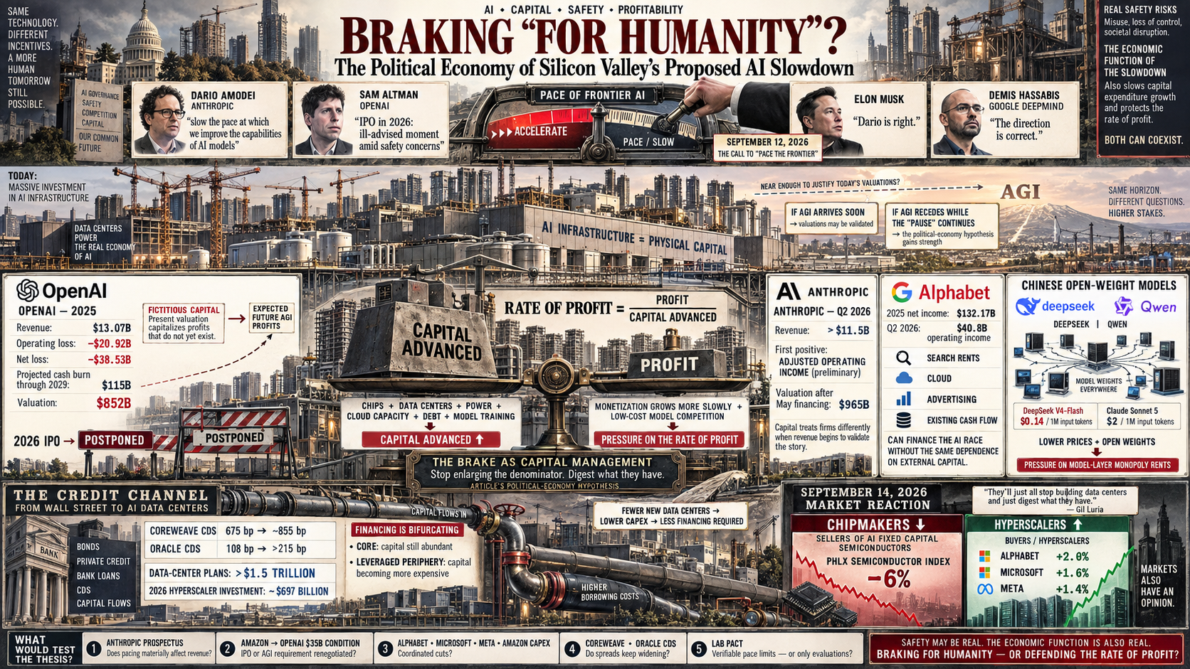
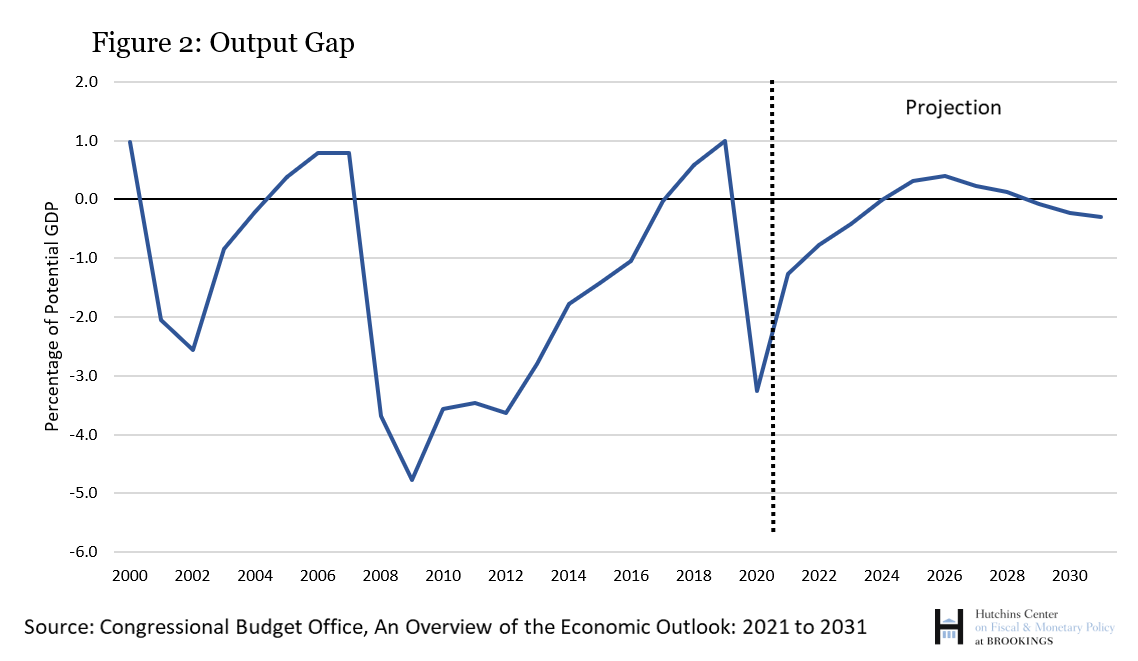


Capitalism, socialism, and the State
Why is it said that the technological level for such a matter does not appear to exist (at least not in a generalized form in every society—and that is a detail of vital importance both analytically and practically)? The answer is related to the refutation of another idea widely disseminated throughout the last century and regarded by many unwary people as the irrefutable scientific-technical proof of the impossibility of Communism: namely, that socialist and even communist social relations of production existed in the Union of Soviet Socialist Republics (depending on which “enlightened” person one happens to be speaking with). When capitalist social relations of production are discussed, it is possible to define them well (to situate them within a general and relatively precise theoretical framework—the precision will vary according to the aspect of reality analyzed and/or the theoretical framework employed by the researcher, which is the meaning of “well-defined” in Pure Mathematics). Does the same occur with “socialist” and/or “communist” social relations of production? Let us briefly review the theoretical-historical and empirical-historical evidence.
The work of Marx and Engels centers on a systematic critique (a systematic analysis oriented toward transforming reality) of the capitalist system of political economy, and there are only a very few and very brief passages in which Marx and Engels discuss some future non-capitalist mode of production (considering their mature works, beginning in the temporal neighborhood centered around the publication of The Poverty of Philosophy—the immediately preceding and following publications). In particular, in Volume II of Capital, Marx lays out rudimentary guidelines for an economic policy concerning surpluses and deficits of fixed assets in a society without private ownership of the means of production and without paper money (let no one imagine Tinbergen’s On the Theory of Economic Policy or anything of the sort; it is a paragraph of a few lines). Engels, in Anti-Dühring (a book positively cited in Lewontin and Levins’s The Dialectical Biologist—which contains in its opening pages a dedication to Friedrich Engels that reads, “To Friedrich Engels, who got a lot of things wrong but got what mattered right”—as well as in other works), argues that the law of value initially ceases to govern only labor power (under socialism) and subsequently the other commodities as well (under communism), being replaced in both cases by a new law according to which the value of commodities is determined by the social needs they satisfy; Engels also develops arguments clearly reinforcing this direction concerning the validity of the law of value in Socialism: Utopian and Scientific.
One cannot deny the furious anti-Marxists and anti-communists roaming about (and they are so dangerous because if they do not understand what Marxism is, still less do they understand what Socialism and Communism are) that the central cell—the progressive extinction of the law of value—exists and is defined. Yet surely even they cannot deny not only that it is minimally defined, but also that there is an enormous difference between a minimal cell and an organism functioning as a self-organized system (a phenomenon appearing in complex systems studied in the mathematical theory of complexity and consisting in the configuration of an order resulting from the interaction among the elements of an initially disordered system—the social state resulting from the resolution of crisis and the transition from one mode of production to another). As an example, the amount of time that elapsed before the first cell initiating life on Earth (since statistical simulations probabilistically indicate that this is how it happened) became a biological system as such was certainly not short.
Moreover, what social relations of production were implemented in the Soviet Union? Was labor power remunerated according to the social needs that it satisfied? What scientific-statistical methodology (and here the role of technological level begins to become visible) did they use to quantify those needs—which are not merely material but also spiritual[3], as Marx makes clear in his Economic and Philosophic Manuscripts of 1844? There was no private ownership of the means of production by persons considered as members of civil society, but there was paper money (where instead there should have existed some well-defined system of equivalence among commodities not subject to artificial fluctuations—not subject to price variation, since paper money and speculation do not exist—that faithfully reflected in exchange relations the technical conditions of production of the commodities being exchanged) and there was state private property (because it is a fact that members of the Communist Party did not live in the same way as the people—even so, the people had greater material dignity than under Western capitalism then and now, although the spiritual dimension remained unresolved; and greater material dignity was hardly detrimental to the people). Thus classes existed insofar as the enjoyment of the social product did not belong to those who produced it—this is the fundamental characteristic—but to the Soviet political class, which underwent bourgeoisification and transformed the Soviet State (beginning with Stalin) into what Marx described as political power, namely, “the organized power of one class for oppressing another” (in classless societies the State is merely an administrator; organs of war directed toward political—class—repression such as police and army do not even exist, because without class antagonisms political power also ceases to exist). This was so even though oppression in the material plane was far less forceful and intense than in the West, while ideologically it was less subtle—the West is more elegant in its methods; one need only ask Merkel about the microphones installed in her office by the Government of the United States that produced a diplomatic incident some years ago—and even foreign actors appeared near the collapse of the Soviet Union, for example the bank David Rockefeller opened in Moscow’s Red Square (which does not belong to the set of “conspiracy theories”; it is a well-documented fact that an elementary web search can verify).
Evidently, what existed in the Soviet Union was State Capitalism, a variant of the capitalist mode of production in which, as Borísov et al.’s dictionary of Political Economy states, it “constitutes a means of struggle against foreign capital, uproots the economic roots of its domination, helps strengthen and develop the national economy. The state sector increasingly stimulates the rapid rise of the productive forces and creates the economic premises for those countries to embark upon a non-capitalist path of development. In the period of transition from capitalism to socialism, state capitalism represents a special form of subordinating capitalist enterprises to the dictatorship of the proletariat, established in order to prepare the conditions for the socialist socialization of all production.” It may also be mixed in the sense that foreign private enterprises coexist with it (while their power over national society is limited) and/or in the sense that private ownership of the means of production is shared by the capitalist State together with domestic or foreign private enterprises (the latter is the case of Cuba, for example), while a case combining the types of state capitalism just mentioned is what occurs in Venezuela.
All this without yet mentioning that capitalism underwent an extremely extended process of birth, since its economic development preceded by centuries its political consolidation as the dominant mode of production. Medieval boroughs, commercial expansion, mercantile accumulation, and later manufacture prepared the material conditions of the new society over several centuries (a process traceable from the High Middle Ages and which long before 1789 had reached a degree of development sufficient to distinguish the bourgeoisie clearly as a historically ascending class). Nevertheless, it is reasonable to locate its decisive political crystallization in the French bourgeois revolution of 1789 and, as the emblematic milestone of that process, in the storming of the Bastille on July 14. What occurred there was not capitalism appearing out of nowhere—it had existed for a long time and was already developed and diffused to varying degrees throughout the known world of the time—but rather the great bourgeoisie decisively conquering political power and beginning consciously to transform institutions in accordance with the needs of the new social relations of production, a process subsequently expanded across much of Europe, including through the Napoleonic Wars. The date 1789 therefore expresses the political crystallization of a much longer material transformation, not the instantaneous birth of capitalist relations.
Of course, the advance of the new mode of social production was not linear. It is well known that France subsequently returned for a considerable period to constitutional monarchy because the feudal class temporarily regained power. Nor has it yet been mentioned that the Soviet Union found itself threatened by the West (not merely militarily—the fundamental factor driving it into the arms race—but ideologically as well—one of the factors determining the need to enter the space race), so the planning of its entire economic and social development had to be oriented under these two major constraints. It is no secret among those who knew the Soviet Union that calculations were still being made with abacuses in supermarkets while the country competed on equal footing with the United States in the space and nuclear races (even surpassing it in many respects, obviously at a high cost). In this sense, neither has it been mentioned that there are indications of substantial Soviet financial indebtedness to Western capital during at least the final period of its existence, precisely in order to finance the arms and space races.