“Is that to say we are against Free Trade? No, we are for Free Trade, because by Free Trade all economical laws, with their most astounding contradictions, will act upon a larger scale, upon the territory of the whole earth; and because from the uniting of all these contradictions in a single group, where they will stand face to face, will result the struggle which will itself eventuate in the emancipation of the proletariat.”
Karl Heinrich Marx · Marx-Engels Collected Works, Vol. VI, p. 290
General Conceptual Foundations of Experimental Block Designs
Local control, randomization, and combinatorial structure: from complete blocks to treatment information.
José Mauricio Gómez Julián
Original publication: · Revised:
1. Comparing treatments under heterogeneous conditions
Comparing treatments requires conditions in which their differences can be interpreted. A field has areas of unequal fertility; animals from the same litter share a background; a machine changes between working days. When these differences become mixed with treatment response, comparisons lose precision. Block designs use prior information about this heterogeneity to construct local comparisons.
The main question is which treatments produce different responses. The blocking factor represents another relevant source of variation: area, litter, batch, or working day. A block brings together units that are relatively similar with respect to that source; treatments are randomly assigned within it. Homogeneity concerns relevant attributes and never means that the units are identical. [1]
A completely randomized design can be valid in a heterogeneous collection of units. However, part of its residual error may reflect differences that suitable blocking could explain. If the blocking factor explains little, any precision gain may be small or offset by the use of degrees of freedom.
2. Unit, treatment, block, and replicate
Experimental vocabulary: four objects worth distinguishing
Object
Meaning
Agricultural example
Experimental unit
Smallest unit assigned a treatment as a whole; its subsamples do not receive separate assignments.
A plot assigned a fertilizer.
Treatment
Condition or combination of conditions whose response is to be compared.
One of four formulations: A, B, C, or D.
Block
Units grouped before treatment assignment according to a relevant source of variation.
A strip with relatively homogeneous fertility.
Treatment replicate
Application to another experimental unit; independence depends on the design.
Treatment A applied to a separate plot in each block.
Subsample
Additional measurement within the same experimental unit.
Several plants measured in one plot.
Measuring ten plants in one plot does not provide ten independently randomized plots. Subsamples can improve measurement of that unit, but treating them as independent replicates creates pseudoreplication and overstates the experimental information.
In a multicenter clinical trial, a center may define a randomization stratum and enter the analysis. This does not imply that each center is a complete block with just one patient per treatment. Blocking on prognostic characteristics should also be distinguished from permuted blocks used to balance assignments during recruitment.
3. What is randomized and what is modeled
Randomization is an assignment procedure. Fixed and random effects are model formulations. Statistical independence describes probabilistic relationships. Linear independence describes relationships among vectors. Each concept answers a different question.
Random assignment: treatment positions are randomized within each block, subject to the design restrictions. With four treatments used once each, assignment is a permutation: allocating one treatment to a plot restricts the choices for the others.
Fixed effects: inference concerns the particular levels included, such as four formulations deliberately selected for comparison.
Random effects: a population of levels and a distribution of their effects are represented. For blocks, a possible model is βj ∼ N(0, σB2) when selection and the inferential objective justify it. [2]
Treatments can be randomly assigned while their effects are modeled as fixed. Assignments may be generated independently between blocks even though they are constrained within each block. This does not establish error independence: spatial proximity, repeated measurements, or interference between units can introduce dependence.
4. Gradients, means, and variances
Systematic differences between blocks may change the expected response without changing residual variance. Three objects should be separated: the mean function, the variance function, and the dependence structure. An additive block effect changes the first; modeling heteroscedasticity changes the second; a spatial or temporal covariance structure changes the third.
Three distinct questions about heterogeneity
Object
Question
Possible representation
Mean
Does the expected level change between blocks?
E(Yij) = μ + τi + βj
Variance
Does error dispersion change?
Var(εij) = σj2
Dependence
Do two units share residual information?
Cov(εij, εi′j′) ≠ 0
Homoscedasticity means constancy of the relevant variance; heteroscedasticity means that it varies. Homogeneity of variance across groups is a common formulation of the former. These properties are not exclusive to any single data structure and must be defined relative to the model and the conditioning involved. [3]
01 · Spatial gradient
∇f(x, y) = ( ∂f/∂x, ∂f/∂y )T
If f represents a differentiable scalar field of fertility, its gradient collects the partial derivatives. It points toward the greatest local increase; its magnitude measures the maximum rate per unit distance. It is not, by definition, a variance gradient. [4]
If fertility changes mainly in one direction, blocks may be narrow along that direction and extend approximately along similar levels. Actual placement requires knowledge of the field. Categorical factors, such as litter or batch, require no derivatives.
Batabyal, Sarkar, and Mandal studied radish in established fertility gradients with NPK and farmyard-manure treatments. Their work provides a material context for controlling heterogeneity; the numerical example below is an independent teaching construction. [5]
· · ·
5. The randomized complete block model
In the classical design used here, there are v treatments, b blocks, and one unit for every treatment–block combination. Each block contains all treatments exactly once: k = v. Thus, the total number of observations is n = vb, and each treatment has b replicates. Complete designs with additional within-cell replication also exist; we explicitly use one observation per cell.
02 · Additive model
Yij = μ + τi + βj + εij
Yij is the response from the unit assigned treatment i in block j; μ is the overall mean; τi is the treatment effect; βj is the block effect; and εij is the deviation unexplained by those terms.
For identifiable parameters under sum-to-zero coding, impose ∑iτi = 0 and ∑jβj = 0. Reference-level coding is another option. Redundancy in a coding scheme does not mean that a treatment is scientifically irrelevant: it means that some parameters need constraints to have a unique representation.
03 · Global treatment hypothesis
H0: τ1 = ⋯ = τv = 0
Under sum-to-zero coding, this is equality of treatment means in the additive model. Rejection indicates that they are not all equal; it does not identify which pairs differ.
Specific comparisons require estimates, intervals, and multiplicity adjustment where appropriate. With shared random block effects, responses in the same block can be marginally correlated; conditional error independence is a separate matter. The model must therefore match the intended level of inference.
6. From field layout to data: a complete example
Consider four fertilizer formulations A, B, C, and D, three blocks with increasing fertility, and twelve plots. The response is a teaching yield index in arbitrary units. The assignments below illustrate three possible within-block permutations; they are not the output of the optional randomization in the R code.
Figure 1 · Field organization
Each cell is a plot; letters identify treatments, not outcomes.
Block
Position 1
Position 2
Position 3
Position 4
B1Lower fertility
C
A
D
B
B2Medium fertility
B
D
A
C
B3Higher fertility
D
C
B
A
Original schematic. Fertility changes mainly between rows; each row contains all four treatments. Shading identifies levels without relying exclusively on color. Fertility is not assumed identical across all plots in a row.
Simulated data, reordered by treatment for readability
Block
A
B
C
D
Mean
B1
18
22
25
29
23.50
B2
28
31
36
39
33.50
B3
37
42
45
50
43.50
Mean
27.67
31.67
35.33
39.33
33.50
The overall mean is 33.50. Successive block means differ by ten units. Under sum-to-zero coding, estimated block effects are −10, 0, and 10; treatment effects are approximately −5.83, −1.83, 1.83, and 5.83. These estimates come from simulated data and do not represent a real agricultural trial.
04 · Fitted response and residual
Ŷij = Ȳi· + Ȳ·j − Ȳ··; eij = Yij − Ŷij
For A in B1, the prediction is 27.6667 + 23.5 − 33.5 = 17.6667. The observed value is 18, giving a residual of approximately 0.3333. The model separates the block level from the difference attributed to treatment.
05 · Orthogonal decomposition
SSTotal = SSTreatments + SSBlocks + SSError
In this complete, balanced design with no missing observations, treatment and block sums of squares separate orthogonally. This expression does not justify carrying the same calculations unchanged into an incomplete design.
06 · Components and F test
SST = b ∑i(Ȳi· − Ȳ··)2; SSB = v ∑j(Ȳ·j − Ȳ··)2 SSE = ∑i,jeij2; FT = [SST/(v−1)] / [SSE/((v−1)(b−1))]
The multipliers b and v count the observations contributing to each mean. Dividing a sum of squares by its degrees of freedom gives a mean square. Under the null hypothesis and the normal additive assumptions, the treatment ratio follows F with v−1 and (v−1)(b−1) degrees of freedom.
ANOVA for the additive block model · rounded values
Source
SS
df
MS
F
Treatments
224.3333
3
74.7778
168.2500
Blocks
800.0000
2
400.0000
—
Error
2.6667
6
0.4444
—
Total
1027.0000
11
—
—
For treatments, F(3, 6) = 168.25 and p ≈ 0.00000353. This indicates incompatibility with equal means under the model; it does not establish that every assumption is true or measure practical importance by itself. The mean difference D−A is approximately 11.67 units. Its unadjusted 95% t confidence interval is approximately [10.33, 13.00], using standard error √(2MSE/b) and six degrees of freedom. This interval concerns that contrast under the stated assumptions.
What happens when blocks are omitted from these same data
Analysis
Error MS
Error df
Treatment F
p
Treatments only
100.3333
8
0.7453
0.55468
Treatments + blocks
0.4444
6
168.2500
0.00000353
7. Assumptions, diagnostics, and limitations
Additivity: the model assumes constant treatment differences across blocks. With one observation per cell, including all treatment–block interactions saturates the twelve observations and leaves zero residual degrees of freedom. Unrestricted interaction cannot be separated from pure error.
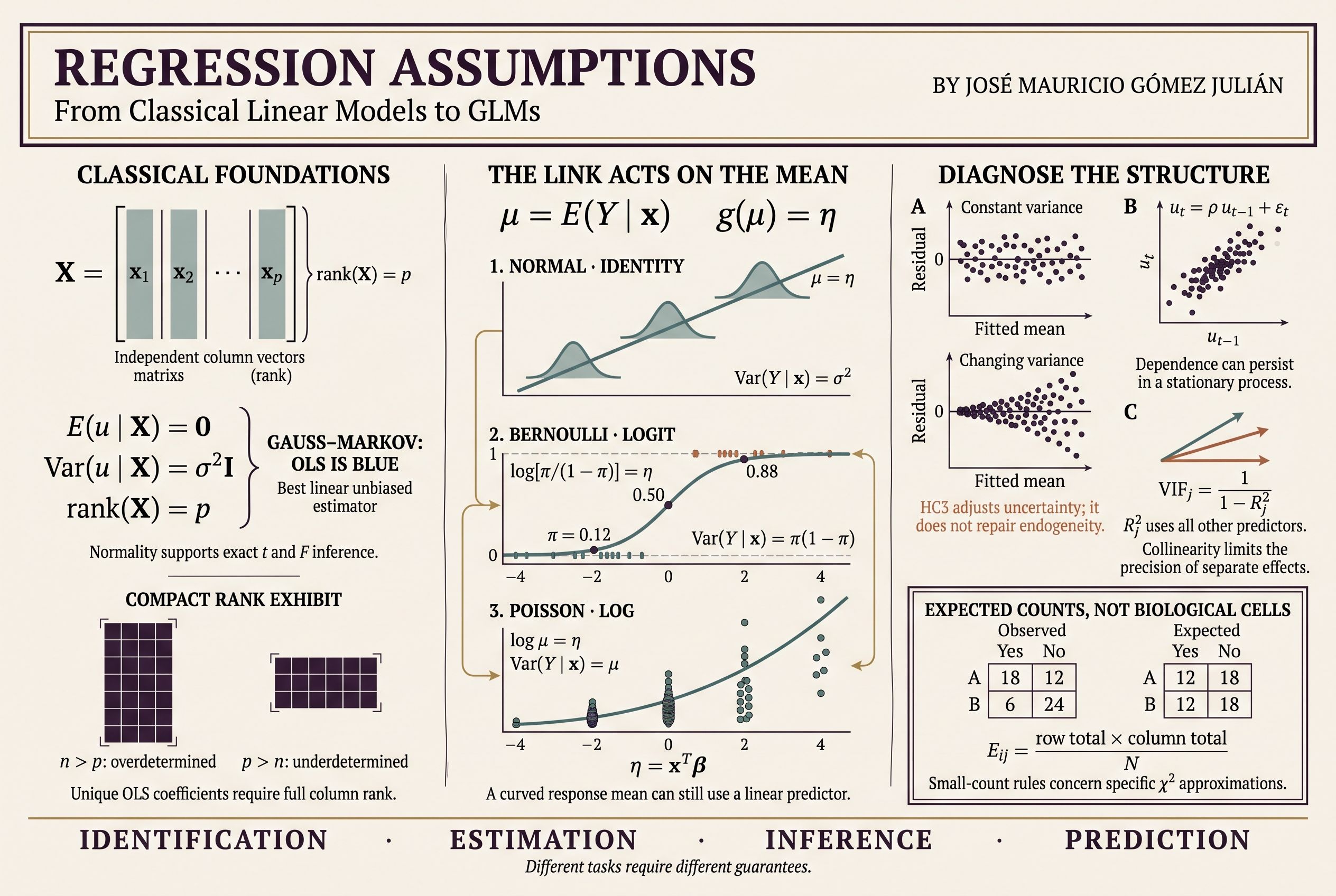
Errors: classical normal ANOVA assumes zero-mean errors, common variance, and independence at the appropriate level. Normality supports the exact F distribution; randomization also supports its own inferential approaches.
Diagnostics: examine residuals against fitted values, treatments, blocks, and the actual run order; use a Q–Q plot and assess spatial patterns when relevant. Diagnostics based on twelve observations have limited power. [6]
Interference and measurement: fertilizer runoff, contagion, or instrument drift can violate comparison conditions. Blocking requires operational measures alongside the statistical layout.
Missing observations: retain the model structure and reassess estimability and sums of squares. The balanced ANOVA table above no longer applies automatically.
Unequal variances may call for generalized least squares or explicit variance structures; dependence may call for covariance structures or mixed models. A transformation requires a substantive interpretation. With few experimental units, robust standard errors are not an automatic remedy either.
Replication, the number of blocks, and the minimum effect of interest should be planned before the trial. Observed significance does not replace a prospective assessment of precision or power.
· · ·
8. When a block cannot contain every treatment
A complete block may become too large to remain homogeneous, or there may be too few comparable units. With twenty treatments and capacity for four units per block, each block contains a subset. This leads to incomplete designs: their structure must support block-adjusted comparisons even when two treatments do not appear together in every block.
Experimentally, a block groups units. In the combinatorial representation of a binary design, it records the set of treatment labels present. This change of representation should be explicit; blocks are not necessarily regions of a probabilistic sample space.
Properties that can be combined without being equivalent
Term
Operational definition
Complete / incomplete
Each block contains all treatments / only a subset.
Binary / nonbinary
A treatment occurs at most once / can repeat within a block.
Equireplicate
All treatments have the same total number of assignments in the experiment.
Proper or uniform
All blocks have the same size.
Simple
No two blocks have the same treatment composition.
Equireplication does not mean equal repetition inside every block. A nonbinary design can also be equireplicate. Repeating a block composition can contribute new observations; it is not equivalent to algebraically duplicating identical information.
9. BIBD: balance through counting
A balanced incomplete block design, BIBD, is binary, has blocks of common size k < v, replicates each treatment r times, and places every treatment pair together in λ blocks. We use the nontrivial convention 1 < k < v and λ > 0.
The five parameters
Symbol
Meaning
Minimal example
v
Number of treatments
3
b
Number of blocks
3
k
Units per block
2
r
Total replicates per treatment
2
λ
Shared blocks for every pair
1
07 · An explicit BIBD
B1 = {A, B}; B2 = {A, C}; B3 = {B, C}
This is a second example, separate from the complete experiment with four fertilizers. Each block contains two separate units: A and B are not jointly applied to one unit. Positions within a block must be randomized.
There are six assignments: A, B, and C each occur twice. The three pairs AB, AC, and BC each occur together exactly once. Direct enumeration establishes the existence of the design with these parameters.
08 · Counting incidences
vr = bk
Counting by treatment gives v groups of r occurrences; counting by block gives b groups of k units. Both count the same assignments: 3×2 = 3×2 = 6.
09 · Counting pair occurrences
r(k − 1) = λ(v − 1)
Fix treatment A. In each of its r blocks it has k−1 companions. Equivalently, it meets each of the other v−1 treatments λ times. In the example: 2×1 = 1×2.
These equalities and integer parameters are necessary but not sufficient for every proposed parameter set. A nontrivial BIBD also satisfies Fisher’s inequality b ≥ v. Proposed parameters require an explicit construction or an applicable existence theorem. [8]
10. From incidence to statistical information
Let rows represent treatments and columns represent blocks. Entry nij counts the units in block j assigned treatment i. In a binary design it is zero or one. An incidence structure records membership; it requires neither distances nor a metric.
Figure 2 · Incidence matrix N
B1 = AB · B2 = AC · B3 = BC
Treatment
B1
B2
B3
Row sum r
A
1
1
0
2
B
1
0
1
2
C
0
1
1
2
Column sum k
2
2
2
6
One indicates presence and zero absence. The bottom-right corner is the total number of assignments, not a block size. This original figure uses the declared orientation of N.
10 · Concurrence matrix
NNT = (r − λ)Iv + λJv
For a BIBD, the diagonal of NNᵀ contains r and the off-diagonal entries contain λ. I is the identity and every entry of J is one. Here the diagonal is 2 and the other entries are 1. [9]
The product counts shared blocks: for A and B, multiply their incidences in corresponding blocks and sum. Only B1 contributes one. N records treatment–block incidence; the model matrix X has one row per observation and columns for model parameters. They are not interchangeable.
11 · Treatment information adjusted for blocks
C = R − NK−1NT
For the additive homoscedastic fixed-block model with equally weighted observations, R = diag(r₁,…,rᵥ) and K = diag(k₁,…,kᵦ). C is the adjusted information matrix, apart from the factor 1/σ². Each kⱼ must be positive.
This expression follows by eliminating block parameters from the normal equations. For a BIBD, R = rI and K = kI. Substituting the concurrence identity and using r(k−1) = λ(v−1) gives:
12 · Information and uniform precision
C = (λv/k)(Iv − Jv/v)
In the example, C = (3/2)(I₃−J₃/3): its diagonal is 1 and its other entries are −1/2. Its eigenvalues are 1.5, 1.5, and 0. The zero corresponds to the common level; the two positive values support contrasts among three treatments.
On the contrast space, C acts as multiplication by λv/k. Thus the intrablock analysis gives Var(τ̂i−τ̂h) = 2kσ²/(λv) for i ≠ h. Here it is 4σ²/3. Equal precision for all pairs follows from the structure under these assumptions; combinatorial balance and heteroscedasticity are different properties.
· · ·
11. Partial balance and further extensions
PBIBDs organize treatment pairs into association classes; their concurrence counts can be λ₁, λ₂, and so on, depending on class. An association scheme imposes additional regularity on these relations: grouping pairs by frequency alone is insufficient. Their relation matrices form an algebra used to investigate structure and precision. Connections with permutation groups exist, but an association scheme is not simply a group. [10]
As an original example, take B1 = AB, B2 = BC, B3 = CD, and B4 = DA. Each treatment occurs twice and each block has size two. Adjacent pairs in the cycle occur together once; AC and BD never occur together. This is a connected two-class design—neighbors and opposites—rather than a BIBD. Opposite pairs are compared indirectly.
For this cycle, C has eigenvalues 0, 1, 1, and 2. Under the same intrablock model, the variance of a difference between neighbors is 1.5σ² and between opposites is 2σ². This derivation shows what can change with partial balance: pairs need not have equal precision.
Alpha, lattice, cyclic, resolvable, unequal-block-size, and unequally replicated designs address different restrictions and can share properties. Choosing among them requires defined comparison objectives and efficiency criteria; no label guarantees optimality in every setting. Dey’s monograph provides a specialized treatment of these families. [11]
13 · Intrablock efficiency of a BIBD
e = λv/(rk) = v(k − 1)/[k(v − 1)]
In the equireplicate homoscedastic case, contrast information is compared with an ideal reference having the same replication r and residual variance. Here e = 3/4: variance is 1/e = 4/3 times that of the reference. This comparison holds σ² constant; it does not contradict blocking reducing residual error relative to omitting real heterogeneity.
Variance balance concerns equal precision of pairwise contrasts under a model. Efficiency balance concerns canonical efficiency factors relative to a specified reference. In the BIBD above, all contrast efficiency factors coincide. With unequal replication or block sizes, definitions and normalization require greater care; these concepts should not be equated without conditions.
12. Local control as the material organization of comparison
Blocking allows experimental objectivity to be understood as an organized practice. Units enter experiments with material conditions and prior histories. Deciding which differences to record and how to distribute treatments determines which comparisons the experiment can support and with what precision.
From a materialist interpretation, statistical abstraction is constructed through concrete operations: delimiting plots, identifying litters, recording batches, assigning conditions, and measuring responses. A model preserves certain determinations of this process and concentrates others in its error term. The distinction among treatment effect, block effect, and residual should be assessed against the mechanism under study.
An attribute is secondary relative to a particular question, rather than necessarily to every investigation. Fertility can be a source of variation controlled when formulations are compared, or the main object of another study. It can also modify their effects, making interaction a research question.
This epistemological reading is an interpretation of the procedure. The definitions of balance, rank, and estimability retain their specific mathematical conditions. Their articulation with a philosophy of science becomes stronger when it explains verifiable experimental decisions and limitations.
13. Reproducing the analysis in R
The following code uses base R only. It reconstructs the twelve observations, fits both models, and checks BIBD incidence. The table is ordered by block and treatment; this is not a temporal run order.
dat <- data.frame(
  block = factor(rep(c("B1", "B2", "B3"), each = 4)),
  treatment = factor(rep(c("A", "B", "C", "D"), 3)),
  response = c(18, 22, 25, 29, 28, 31, 36, 39, 37, 42, 45, 50)
)

unblocked <- lm(response ~ treatment, data = dat)
blocked <- lm(response ~ treatment + block, data = dat)
anova(unblocked)
anova(blocked)
aggregate(response ~ treatment, dat, mean)
confint(blocked)  # coefficient intervals, not all pairwise contrasts

N <- rbind(A = c(1, 1, 0), B = c(1, 0, 1), C = c(0, 1, 1))
colnames(N) <- c("B1", "B2", "B3")
N %*% t(N)
C_info <- diag(rowSums(N)) - N %*% diag(1 / colSums(N)) %*% t(N)
eigen(C_info, symmetric = TRUE)$values
In the full ANOVA for these balanced data, treatment and block terms are orthogonal: their order does not change their sums of squares. In incomplete or unbalanced designs, hypotheses and adjustments must be specified; a sequential sum of squares is not automatically an effect adjusted for every other term.
Intervals from confint() refer to the model parameterization and are not all pairwise comparisons. Diagnostics and their limitations should accompany calculation. The additional R file includes numerical checks and an independent prospective randomization, without changing the figure or retrospectively attaching a seed to it.
14. Criteria for designing and reporting the experiment
Define the response, the minimum relevant effect, and the actual experimental unit.
Choose blocking factors using knowledge of the process and record how blocks were formed.
Check available units, block sizes, replication, and connectedness.
Generate and retain random assignments before applying treatments.
Plan for interference, missing units, repeated measurements, and execution differences.
Choose a model consistent with assignment, dependence, and the population of inference.
Report effects and uncertainty, assumptions, diagnostics, and reproducible data.
Experimental precision begins with how comparisons are organized.
A sound block design connects knowledge of the phenomenon, random assignment, and mathematical structure. Complete blocks provide direct, balanced comparisons; incomplete blocks require organized incidence and estimability. In both, the scope of the conclusion depends on the conditions actually constructed.
References and specialist reading
The counting arguments, data, and numerical derivations of the examples are developed in this article. The sources below support its concepts and provide further reading.
Peter J. Cameron (2012).Balanced and variance-balanced designs. 6th Workshop on Statistics, Mathematics and Computation, Covilhã; incidence and concurrence matrices.
Peter J. Cameron (2003).Association schemes. The Encyclopaedia of Design Theory; definition, matrix algebra, and partial balance.
Aloke Dey (2010).Incomplete Block Designs. Texts and Readings in Mathematics, 57. Hindustan Book Agency; international edition: World Scientific.
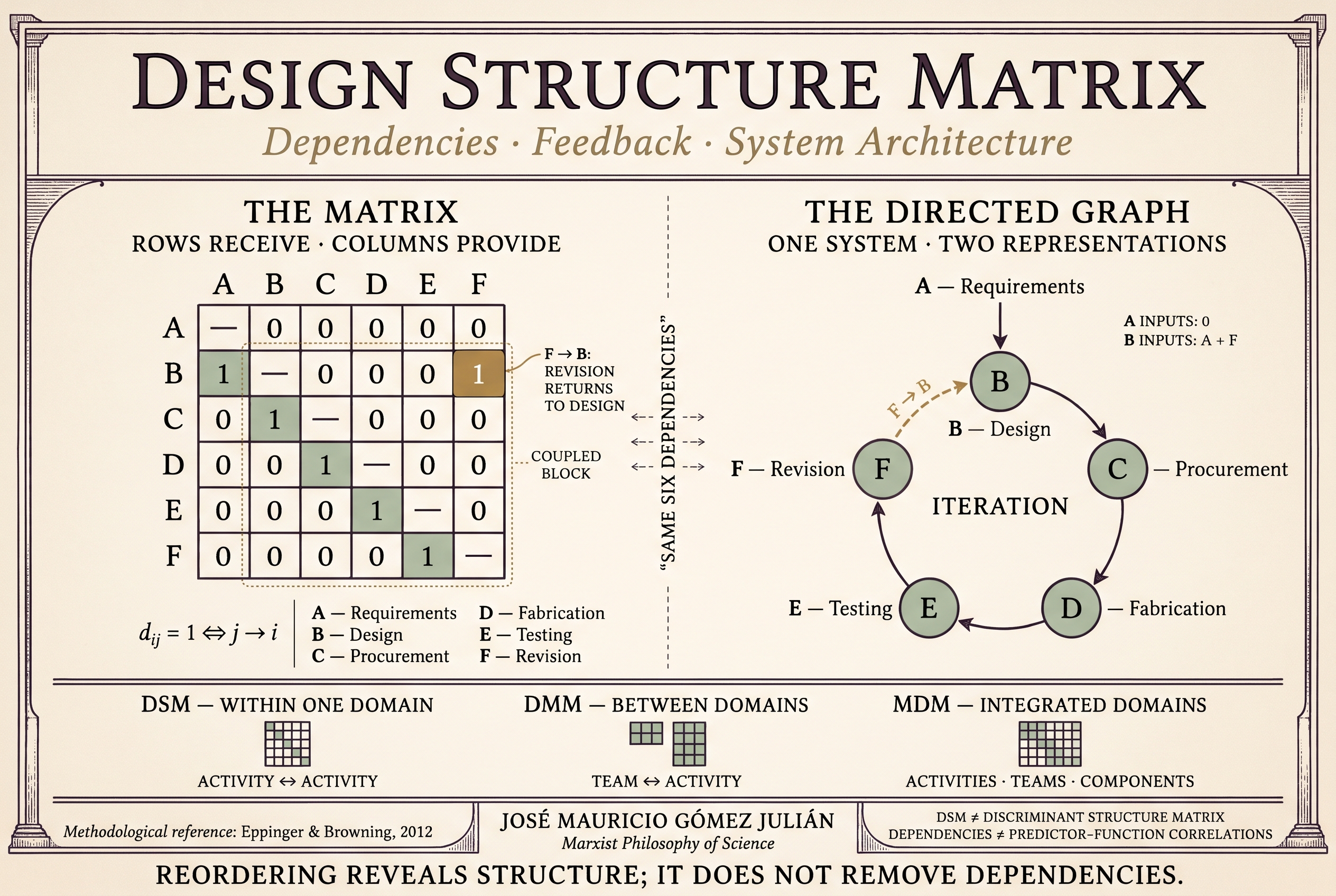
Understanding a system requires identifying both its components and the relationships that make its operation possible. A Design Structure Matrix, or DSM, organizes these dependencies in a square representation: each element appears once as a row and once as a column. Its pattern of marks reveals a relational architecture that a simple inventory of parts would leave hidden. [1]
In a product DSM, elements may be components; in an organization, teams; in a process, activities; and, at a finer level, design parameters. The chosen relationship must be specified: information exchange, material transfer, physical interfaces, and dependencies between decisions are not interchangeable terms. [4]
A useful question precedes drawing the matrix: what does each element need from the others to perform the function under investigation? If the concern is team coordination, recording spatial proximity may be insufficient; if the concern is a thermal interface, counting messages does not answer the question either.
2. Formal definition and reading convention
D = (dij) ∈ {0,1}n×n dij = 1 ⇔ j → in is the number of elements. For i ≠ j, a value of 1 means that i receives an input from j; a value of 0 means that this relationship is absent in the model.
Throughout this article, the row receives and the column provides. Reading across a row identifies its element’s direct inputs; reading down a column identifies the direct recipients of its outputs. This is the inputs-in-rows, or IR, convention. The inputs-in-columns, or IC, convention conveys the same information through the transpose DT. [3]
Zero must not conceal uncertainty either. If a relationship has not been investigated, keep it as unknown in the evidence register and resolve it before turning the table into a complete binary matrix. A recorded dependency expresses the model’s criterion; it does not, by itself, establish causality.
3. An example: from requirements to revision
Consider the development of a simple device. We distinguish six activities and record only deliveries of information or results required by the receiving activity. This is a hypothetical example; its relationships are defined so that every step can be checked.
Table 1. Example activities and inputs
Code
Activity
Represented direct input
A
Requirements
None inside the defined system.
B
Design
Requirements A and revision results F.
C
Procurement
Design specifications B.
D
Fabrication
Materials or procurement results C.
E
Testing
Fabricated prototype D.
F
Revision
Test results E.
Figure 1. Original teaching example. Arrows indicate information or result delivery; the dashed F→B edge closes the revision cycle.
A→B, B→C, C→D, D→E, E→F, F→B. The cycle is B→C→D→E→F→B.
The F→B edge returns observations to design. A revision may require updated specifications, procurement, or fabrication; the model indicates a structural possibility of iteration without claiming that every step must be repeated in full on every occasion. A receives no inputs from the other five activities because requirements are treated as fixed outside the cycle under analysis.
Table 2. Binary DSM: receiver rows and provider columns
Receiver ↓ / provider →
A
B
C
D
E
F
A · Requirements
—
0
0
0
0
0
B · Design
1
—
0
0
0
1
C · Procurement
0
1
—
0
0
0
D · Fabrication
0
0
1
—
0
0
E · Testing
0
0
0
1
—
0
F · Revision
0
0
0
0
1
—
Row B contains two ones: dBA = 1 and dBF = 1. B receives from A and F. Column B contains one one, in row C: B delivers to C. Cell dBF represents F→B, never B→F under this convention.
The table contains six links and thirty off-diagonal positions. Its directed density is 6/[6(6−1)] = 0.20. This number describes the proportion of recorded relationships; it does not automatically measure project complexity, quality, or difficulty.
· · ·
4. Dependency, independence, and coupling
Table 3. Three basic patterns between two elements
Pattern between i and j
Cells
Local interpretation
No direct link
dᵢⱼ = dⱼᵢ = 0
No direct exchange is recorded between them.
One-way dependency
dᵢⱼ = 1; dⱼᵢ = 0
j supplies i, with no reverse direct link.
Reciprocal coupling
dᵢⱼ = dⱼᵢ = 1
Each element requires inputs from the other.
The absence of a direct link does not imply statistical independence or guarantee parallel execution: indirect paths or shared constraints may exist. In our example, A does not deliver directly to C but does so through B.
Nor does every cycle require a reciprocally linked pair. B, C, D, E, and F form the circuit B→C→D→E→F→B although no pair exchanges directly in both directions. Inspecting only symmetric cells would therefore miss the coupling of the whole group.
5. Reorder without erasing dependencies
The same architecture may appear scattered when its elements are displayed in an uninformative order. The following table uses exactly the same six links but orders the elements as E, A, C, F, B, D.
Table 4. The same DSM in an arbitrary initial order
Receiver ↓ / provider →
E
A
C
F
B
D
E · Testing
—
0
0
0
0
1
A · Requirements
0
—
0
0
0
0
C · Procurement
0
0
—
0
1
0
F · Revision
1
0
0
—
0
0
B · Design
0
1
0
1
—
0
D · Fabrication
0
0
1
0
0
—
Dordered = P Dinitial PTP is a permutation matrix: it changes row and column order consistently. Its rows select, from the initial ordering, the positions needed to obtain A, B, C, D, E, F.
Restoring A, B, C, D, E, F produces table 2. The outlined block corresponds to {B,C,D,E,F}; {A} forms the other block. Within the former, each activity can reach every other activity by following arrows: it is a strongly connected component. Condensing these components leaves a single link: {A}→{B,C,D,E,F}.
Partitioning seeks a block triangular structure that reveals these groups. An acyclic graph admits a topological order that places links below the diagonal under our convention. With cycles, the blocks can be ordered, but a mere permutation cannot produce a strictly triangular matrix. [5]
6. From structure to decisions
Clustering seeks modules with strong internal interactions and fewer external links. Sequencing seeks to expose activity precedences and cycles. These are different objectives: a group that benefits from joint coordination need not be an executable sequence or a strongly connected component. [6]
In the example, the B–F block invites coordination between design and execution. It does not prescribe merging five departments. One concrete intervention would be to agree which observations from F require changes to B and which changes actually require repeating C, D, or E. Assigning owners and deadlines would require additional information.
Tearing selects dependencies to be handled provisionally through estimates or assumptions so that an iteration can begin. For example, a preliminary specification of B may be used while awaiting results from F. The assumption must subsequently be checked; omitting a mark from a plan does not eliminate the physical or informational need it represents. [7]
· · ·
7. Measures, paths, and numerical models
kiin = Σj≠i dij ; kjout = Σi≠j dijThe first sum counts direct providers to element i; the second counts direct recipients of element j. These are binary network degrees, not amounts of work.
The input counts for A–F are (0,2,1,1,1,1); their output counts are (1,1,1,1,1,1). B has more direct providers, although every element has the same number of recipients. Neither count suffices to measure impact: one critical interface may matter more than many routine exchanges.
Under ordinary matrix multiplication, (Dk)ij counts directed walks of length k from j to i. In the example, (D2)CA = 1 through A→B→C. For k = 5, the diagonal is (0,1,1,1,1,1), owing to the five-activity circuit. Walks may repeat vertices; they must not be confused with simple paths or propagation probabilities.
A numerical DSM can record strength, volume, or rework probability, provided that each value has a definition and supporting evidence. An ordinal scale does not authorize every operation appropriate to quantitative measurement. [9]
8. DSM, DMM, and MDM: distinguish the domains
Table 5. Three complementary representations
Tool
What it relates
Example
DSM · Design Structure Matrix
Elements of one domain; a square matrix.
Activity to activity: testing → revision.
DMM · Domain Mapping Matrix
Elements of two domains; it may be rectangular.
Team to activity: who performs testing.
MDM · Multiple-Domain Matrix
Integrates DSM and DMM blocks in a multidomain model.
Activities, teams, and components with their mappings.
This distinction expands the example without mixing entity types in one DSM: activity E can be mapped to the laboratory team through a DMM. Another matrix can record interfaces between device components. Integrating them requires defining the meaning of each block and checking that their identifiers are compatible. [8]
9. Construction, validation, and limitations
State the question. Specify the decision the representation should support and what lies outside its scope.
Define elements and granularity. Avoid comparing a very small task with an entire department without justifying the level of analysis.
Define the relationship. Establish direction, unit, threshold, and observation period; separate relationship types when mixing them would make interpretation ambiguous.
Record evidence. Document the source, date, owner, disagreements, and confidence level for each link.
Check the matrix. Review deliveries and receipts with participants; distinguish confirmed absence from unknown information.
Analyze alternatives. Assess how blocks and decisions change when weights, thresholds, or uncertain links are varied.
Validate the intervention. Compare observed results before and after acting; update the matrix when the process changes.
This sequence is a proposed workflow for the example, not a universal optimization algorithm. In a real application, one might measure whether the agreement between B and F reduces avoidable returns or merely shifts work to other activities.
A six-activity matrix does not itself record durations, staffing availability, costs, conflicting objectives, or historical variation. The same structure can operate very differently under other material capacities or coordination rules. In social systems, an observed relationship requires contextual interpretation; formalizing it does not exhaust its explanation.
The matrix makes dependencies visible; understanding them requires knowing the conditions under which they arise.
· · ·
10. Comparative note: the discriminant structure matrix
The term structure matrix also appears in canonical discriminant analysis, but denotes a different object: a table of correlations between predictors and discriminant functions. SPSS Statistics DISCRIMINANT output uses pooled within-groups correlations. This is not a DSM of dependencies. [10]
zℓ = aℓ1x1 + ⋯ + aℓpxpzℓ is a discriminant score; x₁,…,xₚ are predictors and aℓj are coefficients. Its linear form does not make the procedure ordinary regression: the analysis seeks discrimination between groups. [11]
In IBM’s example, an asterisk identifies each variable’s largest absolute correlation with a canonical function. This is a reading aid, not an automatic significance test. The label “stability” proposed for one function summarizes a pattern in that example; it is not a mathematical property of every second function. [12]
A high loading does not make a function useful on its own either. Structure correlations, function coefficients, and predictive performance must be distinguished. Calling a variable “useless” requires an objective and validation evidence; association mainly with a weak function is insufficient.
11. Reproduce the example in R
The following code uses base R only. It builds D from the edges, calculates degrees, reproduces the arbitrary order, and checks the permutation. It also checks the A→B→C walk and the length-five circuit.
The comments state the convention before data entry. Assertions turn expected results into explicit conditions; larger-network analysis should add strongly connected component procedures and retain evidence for each link.
12. Synthesis
A DSM moves from a list of activities or components to an explicit representation of their dependencies. Its usefulness depends on three agreements: which elements are distinguished, which relationship is recorded, and how its direction is read. On that basis, modules, precedences, and iteration circuits can be identified.
In the example, the matrix and graph express the same six links; permutation reveals the coupled B–F block, while A remains an antecedent outside that cycle. The practical decision is to coordinate and verify the deliveries that sustain the process. Visual order aids interpretation; effective improvement requires intervening in relationships and checking the results.
References and further reading
Eppinger, S. D., & Browning, T. R. (2012). Design Structure Matrix Methods and Applications. MIT Press. DOI: 10.7551/mitpress/8896.001.0001. View source.
Today's edition highlights the escalating tensions in global conflicts, with military actions in Ukraine and the Middle East dominating headlines, while also showcasing technological advancements in AI and robotics that are reshaping security and innovation worldwide.
· · ·
Economy & Politics
Rollo Chino: Hangzhou deploys 182 robotic teams for marathon security
Rollo Chino · single source
Hangzhou deployed 182 robotic teams before dawn to support security during its local marathon. The devices combined humanoid robots, robotic dogs, autonomous vehicles, and drones. These machines collaborated in ground and air patrols, explosive detection, and crowd flow management along the route.
Rollo Chino: China shows ballistic missile impact on US aircraft carrier replica
Rollo Chino · single source
China's state TV CCTV broadcast images of a test in Xinjiang desert where a ballistic missile hit a full-scale replica of a US aircraft carrier. The system used would be a DF-26B anti-ship missile operated by the PLA Rocket Force. The mobile missile can carry conventional or nuclear warheads with an estimated range of 3,000 to over 5,000 kilometers.
RT News: Claims of torture spark accusations of abuse at Ukraine detention facility
RT News · single source
Claims of torture at a National Guard facility near Kiev have sparked accusations that the abuse extends beyond one basement. A protest escalated into clashes with security forces after the discovery of what was described as an unofficial Ukrainian National Guard prison in a private home, where detained men were allegedly being held and tortured. Authorities reported conflicting numbers of detainees.
El Ojo Noticias: US attacked Iranian missile and radar platforms on Qeshm island
El Ojo Noticias · single source
US officials informed CNN and Wall Street Journal that a US fighter jet was targeted by an Iranian surface-to-air missile, after which it attacked the launch platform on Qeshm. Washington also acknowledged attacks on Iranian radar systems, stating they were 'limited and defensive' actions to protect its military assets.
Negocios.com: UK and France prepare 2,800 soldiers to enter Ukraine
Negocios.com · single source
The United Kingdom and France are preparing 2,800 soldiers to enter Ukraine. This deployment signals increased Western military involvement in the region.
RT en Español: Russia's adversaries seek to fracture it at a deeper level
RT en Español · single source
Russia's multinational character has always been a target for its adversaries. This is because Russia's diversity constitutes one of its greatest strengths.
Generación IA: A model 660 times smaller outperforms giants of 72 billion parameters
Generación IA · single source
A study by Yann LeCun, Randall Balestriero and teams from AMI Labs, NYU and Brown proposes a different way to train artificial intelligence: learning to relate two views of the same scene, rather than just predicting the next word.
r/ClaudeAI: Solo Developer Creates Playable Horror Game in Four Days Using AI Tools
r/ClaudeAI · single source
A solo developer built a playable horror level inspired by Silent Hill and Fatal Frame in just four days using Opus 5.5, Godot, and AI-generated 3D assets. The developer used Claude Opus 5.5 for coding, Meshy T2.5 for 3D models, and Nano Banana for images, with an estimated cost of $180 in API usage.
r/claude: Anthropic Reports Possible Dramatically Accelerated Progress in AI Development
r/claude · single source
Anthropic updated its S1 filing stating it may imminently meet its definition of 'dramatically accelerated progress attributable to AI.' However, the company does not anticipate being able to safely use Claude to fully autonomously design successive generations of frontier models.
Bloomberg Technology: Runway's CEO Discusses Generative AI Moving Toward Interactive Worlds
Bloomberg Technology · single source
Anastasis Germanidis, Co-Founder & Co-CEO of Runway, discussed with Bloomberg's Peter Elstrom how generative AI is evolving beyond content creation to create interactive worlds that people can see, shape and experience, during Bloomberg Tech 2026 in London.
Debates at IIPPE 2021: value, uneven development and structural determinations of essence
JOSÉ MAURICIO GÓMEZ JULIÁN
Original publication: September 30, 2021 Revised and expanded edition: November 2, 2026
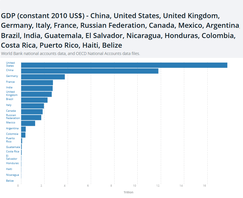
GDP in constant 2010 dollars Comparison across economies. Source shown in the graph: World Bank and OECD.
Introduction: a controversy over relations, mechanisms and measurements
Imperialism poses a problem that cannot be resolved by listing powerful countries. It requires an investigation of how the relations that enable particular capitals to appropriate surplus labour generated in other territories are produced and reproduced. Technology, wages, ownership, credit and state power participate in that reproduction, but their roles cannot be established through a single label.
IIPPE—the International Initiative for Promoting Political Economy—is a pluralistic forum for critical research. Its name refers to political economy, a field of inquiry, rather than exclusively to economic policy, understood as public intervention. [1]
Michael Roberts’s review, published in September 2021, provides the documentary starting point. It connects imperialism, China, financialisation and interest, adding a Colombian study that was not presented at the conference. Our purpose is to reconstruct the underlying problems, examine their mediations and clarify the differences between hypotheses, measurements and conclusions. [2]
Three questions guide the essay: Which social relation is being explained? What mechanism is proposed, and under what conditions? Which observation could test it? Convergent findings can strengthen an interpretation without automatically making the models that generate them equivalent.
I. Background: from finance capital to unequal exchange
A genealogy that neither begins nor ends with one author
Hilferding published Finance Capital in 1910; Luxemburg, The Accumulation of Capital in 1913. Bukharin investigated the internationalisation of capital and its articulation with states; Lenin wrote Imperialism, the Highest Stage of Capitalism in 1916, and the book appeared in 1917. Their contributions constitute a historical controversy, not interchangeable stages of a homogeneous theory. [3, 4, 5, 6]
To study this controversy, it is useful to distinguish corporate concentration, the articulation of banking and industry, capital exports, problems of reproduction and interstate rivalry. An author can illuminate one relation without providing a complete explanation of all the others. Lenin’s centrality does not require attributing absolute priority to him over every Marxist investigation of the world economy.
Emmanuel shifted the discussion towards international wage differences and prices of production. His formulations of 1962 must be distinguished from the French book of 1969 and its English edition of 1972. His proposal integrates international exchange into an inquiry into value and the worldwide distribution of surplus. [7]
Emmanuel: economic assumptions and political implications
In his characteristic formulation, capital mobility and restrictions on labour mobility make it possible to examine a tendency towards equal profit rates alongside persistent wage differences. The question is how these assumptions affect international prices and the distribution of social labour. [7]
Evaluating the argument requires making the time horizon, degrees of mobility, wage determination and price formation explicit. Altering an assumption may alter the conclusion. This does not invalidate modelling: it specifies the explanation’s domain.
The implications for international solidarity deserve their own discussion. A relative distributive advantage for some workers does not automatically turn them into owners of the means of production or eliminate their antagonisms with capital. Conversely, acknowledging exploitation within each country does not require denying international hierarchies. Class position and territorial insertion must be examined together.
Explaining Emmanuel’s reception exclusively through political convenience would replace investigation with imputation. Both political conflicts and theoretical disagreements are recognised here. Controversial attributions—for example, that an author treats capital as an autonomous source of value—require precise passages and contexts; they do not follow from the use of simultaneous equations.
II. Value, surplus value and transfers: distinctions that explain
Production and appropriation are different processes
In Marx’s theory, value concerns socially necessary abstract labour, rather than any individually clocked expenditure of effort. The formation of a general profit rate and prices of production makes it possible to investigate differences between the surplus produced by a capital and the surplus it ultimately appropriates. [8, 9]
For an introductory scheme, assume one turnover and that all the constant capital considered is consumed during the period:
W = c + v + s
Here c is the value of consumed means of production transferred to the product; v, variable capital advanced for labour power; and s, surplus value. The expression organises theoretical categories. Estimation requires deciding which observations represent each term and how labour magnitudes are translated into monetary magnitudes.
e = s / v · r = s / (C + V)
The surplus value rate relates the surplus to variable capital. The profit rate relates a flow of profit per period to the relevant total capital advanced, C + V; this must not be confused without justification with consumed costs, c + v. The rates are comparable only when periods, turnover and valuation conventions are aligned.
A teaching example of redistribution
Consider two capitals of 100 units each, with one turnover, full consumption of constant capital and a surplus value rate of 100%. A uses 70 units of constant and 30 of variable capital; B uses 40 and 60. Their surplus values are 30 and 60. Total surplus value is 90, and the hypothetical average profit rate is 90/200 = 45%. If each realises 45 in profit, A appropriates 15 more than it produced and B appropriates 15 less.
This is a teaching construction, neither a historical estimate nor a universal solution to the transformation problem. Costs are held given to isolate the mechanism; a complete system must also explain input prices. Redistribution does not create the 90 units of surplus value: it changes their appropriation.
What zero-sum means—and what it does not
If Tᵢ denotes a net transfer within an accounting universe that is closed and uses the same unit of valuation, then:
Σᵢ Tᵢ = 0
This identity concerns the distribution of a given magnitude. It does not imply that every economic interaction or expanded reproduction is zero-sum. Production can generate new value; transfers redistribute its appropriation. If the data do not sum to zero, coverage, valuation and statistical discrepancies must be examined before the residual becomes a theoretical conclusion.
Material welfare, the quantity of use values and the magnitude of value must also be distinguished. Productivity gains can increase available goods without proportionately increasing value per unit. “Benefiting from trade” and “appropriating a net transfer of value” are different questions.
III. One concrete essence and multiple structural determinations
Components, common essence and material totality
The components of a totality, represented through equations articulated within a system, may share determinations of a common essence that makes their unity and differences intelligible. This essence is expressed through set-theoretic, topological, differentiable, metric, operational, and historical and dynamical determinations: each makes particular constitutive relations available for investigation. When a correspondence preserves the relations of a defined structure, an isomorphism can be established at that level; equivalence in one determination can coexist with differences in others.
The articulation of components admits an integrodifferential representation when the problem requires rates of change, distributed effects or accumulated memory. Under determinate initial conditions and constraints, interactions constitute an internal structure of a material nature: objective through the efficacy of its relations, dynamic through its reproduction and transformation, and nonlinear where its functional dependencies have that property. The coherence of this articulation includes the compatibility of its relations and equations alongside antagonisms and tensions that can drive its development.
The totality’s structure, generated through component activity, in turn conditions those components’ possibilities of existence, reproduction and transformation. System composition and structural conditioning form a reciprocal relation: interactions produce organisation, and organisation modifies the conditions under which those interactions continue. Emergent properties are explained through this articulation rather than a simple inventory of isolated components.
The laws guiding the investigation of this genesis and reproduction acquire a generalised realisation within a totality with new mediations. The unity and struggle of opposites allows investigation of the constitution and transformation of antagonistic relations and their processes of emergence and self-organisation; the transformation of quantity into quality concerns regime changes, which can be formalised through bifurcations in particular models; and the negation of the negation examines reorganisations preserving and transforming previous determinations. Chemical synthesis provides a concrete example of material reorganisation and the emergence of properties. These connections are developed by specifying mechanisms and conditions: a general dialectical law does not by itself impose an identical functional form, a bifurcation or self-organised criticality on every system.
Integrodifferential composition and reciprocal conditioning
Representing a component through an equation means selecting variables and relations relevant to the problem. Representing the totality must additionally incorporate couplings between components and the restrictions imposed by their organisation. Integration can capture distributed or accumulated effects; differentiation can describe rates of change. Their articulation expresses a concrete possibility for formalising the thesis.
In a domain where differentiable evolution is an appropriate description, reciprocal conditioning can be schematised as follows:
x(t) collects the component states; S(t) represents organisational variables or structural constraints; Ht, the relevant history up to that moment; and θi and Θ, model parameters. The first equation expresses how component behaviour depends on the organised totality. The second expresses how that organisation is reproduced or transformed through component activity. Both must satisfy compatible initial conditions and constraints.
Where accumulated memory needs representation, an integral contribution can be added:
mi(t) = ∫0t Ki(t, τ) Qi(x(τ), S(τ)) dτ
Qi represents the contribution of earlier interactions and Ki their present weighting. This formulation allows investigation of how different histories can modify current possibilities. It is a modelling scheme requiring functions, units and observations to be defined for each application; it does not assert that every system must take this specific form.
The structure is material and objective insofar as the represented relations are effective in the object and do not depend on the investigator’s will. The objectivity of a relation and the adequacy of its mathematical representation are connected but distinguishable questions. Structural reproduction can constrain particular actions while those same actions contribute to sustaining or altering it.
Emergence, nonlinearity and generalised lawfulness
The totality contains relations and capacities that cannot be explained by listing isolated components. Explanation requires investigating their organisation and interactions. A dynamics is nonlinear when its functional dependencies do not satisfy the relevant linearity property; couplings can supply concrete mechanisms for this nonlinearity. Explaining the difference between a totality and the sum of its parts requires identifying these organisational relations.
Generalised lawfulness retains the relation between the system’s genesis and reproduction conditions. The processes constituting a structure subsequently operate within an organisation that modifies their scale, mediations and effects. Continuity of lawfulness can coexist with a transformation of its concrete form of realisation. Sharing general principles does not require using an identical equation at every scale.
In the problem of imperialism, capitals participate in general valorisation relations while their worldwide articulation configures production chains, monetary hierarchies and access to technology and credit. These structural relations condition particular capitals’ reproduction, while those capitals reproduce them through investment, production and appropriation. Moving from the national to the international requires investigating this reciprocity and its historical mediations.
The following layered table specifies the determinations of this articulation; section IV develops the three dialectical laws orienting its interpretation.
What a layered interpretation contributes
Essence can be interpreted as the articulation of constitutive relations that makes an object’s identity and reproduction intelligible. Understanding it requires abstractions, but no single abstraction necessarily exhausts that articulation. Mathematics can specify particular relations; the correspondence between formalism and object requires additional justification.
Interpreting essence as an articulation of structural determinations makes it possible to distinguish the following levels. [10]
Determination
Structural question
Possible formalisation and scope
Set-theoretic
Which elements or states are distinguished?
A set and correspondences; a bijection preserves cardinality, not every additional relation.
Topological
What continuity, neighbourhood and connectedness exist?
A topology; homeomorphisms preserve its structure.
Differentiable
Which smooth variations can be described?
A smooth structure; diffeomorphisms compare that structure.
Metric
How are lengths or distances quantified?
An appropriate metric; isometries preserve the corresponding geometry.
Operational
Which transformations preserve selected relations?
Automorphisms and group actions; Lie groups apply in cases with a compatible smooth structure.
Historical and dynamical
How was the system constituted, and which transitions does it admit?
Evolutions, path constraints and categories of transitions; irreversible histories do not reduce to invertible symmetries.
These layers are articulated determinations of a concrete essence, not six independent substances. Their selection depends on the object. A trade network does not automatically possess a manifold’s topology; an economic inequality does not by itself constitute a mathematical distance. States, relations and observation procedures must be defined in each case.
Adding structure and preserving structure
Equipping a set with a topology differs from establishing a homeomorphism between spaces. Transformations should therefore not be drawn as if they independently created the next level’s structure. For a smooth manifold M with Riemannian metric g, transformations of the object satisfy:
Isom(M, g) ⊆ Diff(M) ⊆ Homeo(M) ⊆ Bij(M)
Preserving the metric imposes additional conditions beyond preserving only differentiable structure; preserving the latter imposes additional conditions beyond topological equivalence. The inclusions are not asserted to be universally strict. Moreover, not every topology admits a smooth manifold structure, and this chain does not classify all mathematical structures.
The same underlying space can admit different geometries
On the upper half-plane U = {(x,y): y > 0}, compare:
gE = dx² + dy² · gH = (dx² + dy²) / y²
The set, usual topology and smooth structure coincide. Gaussian curvature differs: K = 0 for gE and K = −1 for gH. No isometry exists between these geometries. Topological equivalence does not decide metric equivalence.[11]
Curvature does not prevent a global metric from existing. Under the usual assumptions—a smooth, Hausdorff, second-countable manifold—Riemannian metrics can be constructed using partitions of unity. A global metric differs from a global chart, a constant matrix in every coordinate system or a globally Euclidean geometry. [11]
Invariance, identity and historical transformation
An invariant is always relative to a class of transformations. Remaining unchanged under coordinate changes, under isometries or during physical evolution are different properties. Knowing an abstract symmetry group is also insufficient to reconstruct uniquely every structure admitting it.
“Operational essence” can designate the restrictions delimiting particular structurally admissible transformations. This does not identify every change that leaves a system recognisable with an exact symmetry. An organism or an economy can persist through dissipative processes that do not preserve a metric.
For irreversible transitions, a category or semigroup may be more suitable than a group. A groupoid permits partial composition and multiple objects, but requires invertible morphisms: having additional objects does not itself introduce irreversibility. Noether’s connection between symmetry and conservation requires variational dynamics and the corresponding assumptions. [12]
From the national to the international scale
The persistence of wage labour, surplus appropriation and competition between capitals makes common relations across scales a legitimate research question. Currencies, borders, jurisdictions, intellectual property and migration restrictions nevertheless introduce specific mediations. An international structure cannot be obtained merely by multiplying a national structure.
Establishing an isomorphism would require defining the compared structures and constructing a correspondence that preserves their relations. Many applications instead involve aggregations, projections or partial correspondences. Sharing a general law does not prove that components are mutually isomorphic, or that each is isomorphic to the whole.
This qualification retains a decisive dialectical insight: general relations are realised under concrete conditions and can acquire new determinations within a more complex totality. Investigating that articulation requires specifying what is preserved, what emerges and what ceases to be equivalent.
IV. Dialectics, complexity and time: connections with conditions
The three dialectical laws in the constitution and transformation of the totality
The constitution and transformation of the totality are examined through three laws: unity and struggle of opposites, transformation of quantity into quality, and negation of the negation. Their function in this essay is to guide a reconstruction of the material totality’s genesis, reproduction and transformation. Each proposed mathematical relation must show which aspect of this reconstruction it expresses.
1. Unity and struggle of opposites. The terms of a contradictory relation presuppose and condition one another within an organisation, while their tendencies can oppose one another. Inquiry must explain both the reproduction of this unity and the tensions transforming it. In the capital–labour relation, for example, capital’s reproduction presupposes wage labour, but surplus appropriation places participants in antagonistic positions over its distribution and control. The totality is constituted through these relations and imposes conditions on their realisation.
The reference to emergence and self-organisation opens a positive question: how do interactions produce an order which subsequently regulates its own reproduction conditions? A model can investigate feedback and emergent constraints to address it. If self-organised criticality is additionally proposed, the mechanism and properties warranting that specific concept must be identified. The analysis of reciprocal organisation thus connects philosophical explanation with a defined research requirement.
2. Transformation of quantity into quality. Accumulated variations can modify a system’s organisation and possibilities until a different regime is constituted. The problem is to investigate what accumulates, which relations mediate that accumulation and when the relevant quality changes. A bifurcation represents this passage when parameter variation changes a dynamics’ qualitative structure. In political economy, a hypothesis about concentration and market power must establish how changes in magnitude reorganise relations between capitals; accumulating figures alone does not demonstrate that change.
3. Negation of the negation. Transformation can supersede an organisational form through processes which that form itself helped generate. The new organisation preserves determinations of the preceding process while transforming their articulation. This perspective investigates historical continuity within qualitative discontinuity: which relations are displaced, which are preserved and in which new configuration they reappear. It does not assume that every trajectory necessarily advances towards a favourable outcome or repeats an identical cycle.
Chemical synthesis illustrates material reorganisation and the emergence of a compound’s properties. Extending this to a general dialectical law requires explaining the mediations and meaning of the negations in the investigated process. The connection requires determining which relations and processes warrant generalising from each example.
The three laws are articulated within the argument: contradictory relations constitute a unity, variations can transform its organisation, and transformation incorporates a history preserving and modifying previous determinations. Integrodifferential modelling and the layers of essence make particular aspects of this articulation available for investigation.
Scope of the mathematical correspondences
The unity and struggle of opposites directs attention to antagonistic relations; it does not by itself imply that a model exhibits self-organised criticality. The latter requires a dynamical definition and evidence of its properties. Similarly, emergence and non-additivity are insufficient to demonstrate mathematical nonlinearity: the relevant equations, operations or functional relations must be identified.
A bifurcation provides one possible formalisation of particular qualitative changes when dynamics change regime as a parameter varies. Not every qualitative change is a bifurcation in the technical sense. Chemical synthesis can illustrate concrete transformations; identifying it with the negation of the negation would require an independent argument.
Self-similarity likewise does not follow from the existence of relations between parts and a whole. It can be exact, approximate or statistical and must be established through a defined scaling transformation. Dialectical inquiry gains precision when mathematical connections become testable problems.
Temporality and simultaneity in the transformation problem
One axis of Marxist debate contrasts simultaneous valuation of inputs and outputs with interpretations that distinguish moments of valuation. It matters, but does not exhaust the classification of schools. Relations between value and price systems, money, reproduction and distributive closure also matter.
Simultaneous equations can represent conditions within a period or states of a dynamic process; they do not automatically deny time’s existence. A temporal formulation does not become historically adequate merely by introducing a subscript t. It must explain what is inherited, what changes and how periods are connected.
The MELT—monetary expression of labour time—connects labour and monetary magnitudes under a chosen formulation. Its definition, units and valuation date must be declared. Labour hours and money cannot be added as a homogeneous magnitude without such mediation.
Differences between models demand more than observing different numerical results. They require comparison with relevant data, explicit closures and assumptions. Not every methodological controversy has an immediate empirical resolution, nor does comparison with other philosophies of statistics settle this debate by itself.
V. Unequal exchange: theories, indicators and evidence
A map of mechanisms
Approach
Explanatory focus
Question requiring examination
Emmanuel
Wage differences and international price formation under mobility assumptions.
How do results change with mobility, wages and model closure?
Carchedi–Roberts
Transfers estimated through capital composition, surplus value and production prices.
How are theoretical categories translated into national accounts and export sectors?
John Smith
Super-exploitation and the international organisation of production.
How are labour-power reproduction and the location of appropriation observed?
Andrea Ricci
Unequal-exchange measurement and international productive structure.
Which monetary conversions and sectoral aggregations make labour comparable?
Cogliano–Veneziani–Yoshihara
International exploitation, endowments and credit markets in a calibrated model.
What depends on the index’s definition, and what on mechanisms of persistence?
This table proposes reading questions; it does not equate different mechanisms. Indicators classifying some countries similarly may differ in their measured object and causal explanation. [7, 13, 14, 15, 16]
Carchedi–Roberts: measurement and decomposition
The 2021 presentation estimates trade transfers separately from primary income. Its comparison of methods records $600 billion for 2019, equivalent to 1.3% of reference GDP, and $600 billion in primary income for 2017, equivalent to 1.4%. The graph uses each bloc’s own denominator; it is not a homogeneous time series of one combined sum. [13], slides 16–17
Figure 1. Unequal exchange as a share of each bloc’s GDP, 1950–2019. Carchedi–Roberts, 2021 presentation. IC-GDP: imperialist bloc; DC-GDP: dominated bloc. Denominators differ. Series expressed as percentages of each bloc’s GDP.
The positive and negative lines need not have equal percentage magnitudes: the same flow can be divided by different GDPs. Nor should they automatically be equated with the rounded 1.5% in the 2021 account. Reproducing the calculation requires specifying the estimation procedure, year and denominator.
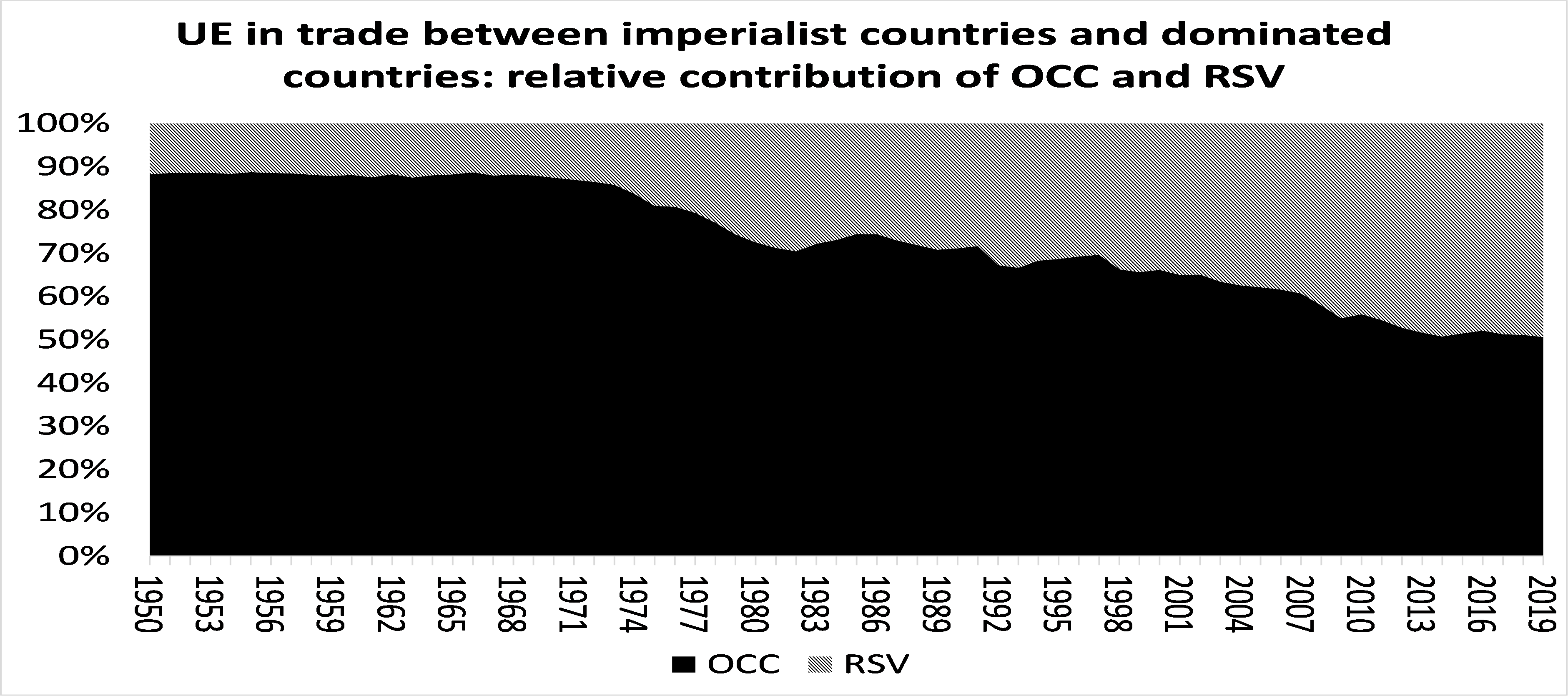
Figure 2. Relative contributions of OCC and RSV to unequal exchange, 1950–2019. Carchedi–Roberts. OCC: organic composition of capital; RSV: rate of surplus value. Shares in a model decomposition, not growth rates.
The decomposition between OCC—organic composition of capital—and RSV—rate of surplus value—belongs to the model. A rising relative contribution does not necessarily mean that the other factor’s absolute contribution is falling. Organic composition is not a direct, universal measure of technological superiority: its relation to productivity depends on techniques, wages, prices and sectoral composition.
Super-exploitation: production organisation and appropriation
Smith emphasises working conditions and wages in global production, challenging the identification of where value is generated with where national accounts record its appropriation. His linked study makes it possible to examine the objection without reducing it to terminology. [14]
The disagreement requires distinguishing criticism of an indicator from denial of all unequal exchange. It also requires avoiding identification of the immediate employer with the sole beneficiary without studying contractual and ownership relations. Subcontracting, commercial control and ownership can articulate successive appropriations. Evaluation must follow the chain and its concrete conditions.
Ricci: transfers per person and units of comparison
Figure 3. Annual transfers per person and percentages by period, 1995–2019. Ricci (2022), table 2. Current dollars and period-average percentages; accessible transcription below.
The figure distinguishes annual amounts per person in current dollars for 1995, 2007 and 2019, and percentage columns for 1995–2019, 1995–2007 and 2007–2019. These percentages must not be presented as growth rates, or the last monetary column mechanically paired with a single annual percentage. [15, 27]
Transcription of figure 3; checked against Ricci (2022), table 2. Positive signs: inflows; negative signs: outflows. Groupings follow the source.
Region
USD/person 1995
USD/person 2007
USD/person 2019
Mean % 95–19
Mean % 95–07
Mean % 07–19
North America
761
1965
2680
3.9
3.7
4.1
EMU
1720
4939
4836
10.3
8.5
12.2
West Europe
2429
7531
6921
12.7
10.6
14.8
East Asia
1984
1766
2540
5.8
5.9
5.7
Oceania
526
2626
3638
7.1
4.5
9.8
China
−196
−810
−426
−14.1
−19.0
−10.0
Russia
−767
−1108
−1850
−29.7
−40.9
−17.2
East Europe
−901
−615
−1309
−14.7
−18.9
−9.9
South America
−269
−472
−490
−6.1
−8.4
−3.9
Central America
−471
−379
−454
−11.9
−13.6
−9.8
Middle East
−1443
−1502
−950
−18.9
−24.8
−12.8
South Asia
−77
−220
−351
−21.5
−20.2
−23.0
Southeast Asia
−463
−1350
−1631
−46.8
−53.9
−40.3
Central Asia
−272
−380
−924
−11.9
−13.6
−9.8
North Africa
−426
−1099
−1034
−30.7
−31.6
−30.4
S. Sahara Africa
−65
−120
−132
−10.0
−11.6
−8.3
In particular, South Asia must not be renamed India; East Asia is not simply Japan; and South America and Central America are not one regional observation. The table reports regions, not individual findings for each country.
In Global locational inequality (2022), table 2 shows that percentages are period averages and monetary amounts are nominal dollars. EMU denotes the European monetary union bloc in that classification. Its regions also need not coincide with states: “China” incorporates Hong Kong, Macao and Taiwan in this statistical aggregation; “Russia” includes other countries, and “Central America” includes Mexico and the Caribbean. These groupings follow Ricci’s statistical classification. Findings must be interpreted according to that territorial coverage. [27]
An international index is not the axiomatic article
Figure 4. Exploiter and exploited countries: basic economy. Exploitation intensity index and wealth per person. Cogliano–Veneziani–Yoshihara’s international model differs from Yoshihara–Veneziani’s axiomatic foundations.
Yoshihara and Veneziani’s article (2018) examines exploitation’s axiomatic foundations. The Dynamics of International Exploitation by Cogliano, Veneziani and Yoshihara (2022) develops a model of international exploitation. Its basic economy assigns China an index of 0.9935: just on the exploiting side of the threshold 1, with the authors advising against a definite conclusion. [16, 17]
The graph relates exploitation classification to wealth per person in a basic economy. An index close to the threshold requires sensitivity analysis. Partial agreement with other studies must not erase classification differences.
VI. China: three questions that must be distinguished
Transfers, mode of production and international power
Roberts’s presentation When did China become capitalist? argues for a trapped transitional economy: it emphasises state direction and planned investment while acknowledging the law of value’s operation. The argument is documented as a position held in 2021, not a classification accepted by all authors. [18]
Dimension
Object of investigation
Relevant evidence
International transfers
Net appropriation under an indicator and period.
Trade, production, primary income, conversion assumptions and sensitivity.
Socioeconomic organisation
Ownership, control, labour and surplus allocation.
Corporate governance, investment decisions, labour discipline, planning and markets.
Imperialist power
International domination and the reproduction of hierarchies.
Credit, monopolies, coercion, institutions, foreign policy and military capacity.
Being a net recipient under an indicator does not by itself establish comprehensive imperialist domination; being a net donor does not exclude relations subordinating third parties. Scale matters: different positions may coexist across sectors, firms, partners and territories.
Sam King examines monopoly over technologically complex activities as a mechanism reproducing international hierarchy. His 2021 book, Imperialism and the Development Myth, frames the question of productive upgrading and its limits. [19]
The review also records Walter Daum’s political objection and different positions from Dic Lo and Cheng Enfu. These interventions are acknowledged as disagreements without attributing to them a demonstration that the review does not provide. [2]
What a growth trajectory cannot decide
Growth, poverty reduction and the capacity to sustain investment require explanation. They do not by themselves identify a mode of production. Connecting them causally with an ownership form would require mechanisms, comparators, periodisation and external conditions; a favourable outcome is insufficient to identify its cause.
It would also be circular to declare that every capitalist economy must reproduce precisely one crisis trajectory and exclude any differing case from the category. A theory must specify tendencies, mediations and conditions, and admit observations capable of challenging its scope.
Dates are decisive. A productivity comparison using aggregate data preceding 2021 does not authorise indefinite descriptions of every Chinese industry as technologically backward. Each conclusion’s scope depends on its period, sectoral disaggregation and supporting sources.
VII. Financialisation: specify the hypothesis before rejecting it
One term, several objects
Research can examine finance’s share of value added, credit expansion, household indebtedness, financial income of nonfinancial firms or shareholder power. Each dimension needs its own indicators. None automatically substitutes for every other dimension.
Mavroudeas challenges finance’s independence from productive accumulation. Rabinovich specifically examines the financial rentierisation hypothesis for US nonfinancial corporations, finding that asset and income composition require a more differentiated interpretation. These arguments have different scopes. [20, 21]
Methodologically, a declining sectoral share can coexist with increasing absolute size. An average can conceal corporate concentration. Changes in value added do not directly equal changes in assets, credit or institutional power. Indicator selection must answer a hypothesis defined in advance.
What the percentages 51.2% and 65.9% measure
This distinction changes the evidence’s meaning. Counting countries measures how widespread a sign of change is; it does not measure the aggregate magnitude of that change or automatically weight countries by economic size. The chosen time window also matters for detecting earlier expansion.
Concluding that financialisation explains deindustrialisation requires temporality, mechanisms and alternative variables. An association between sectoral shares does not itself identify causality. Conversely, rejecting an exclusively financial explanation of crises does not eliminate the roles of credit, collateral and liquidity in their transmission.
VIII. Interest and profitability: structural relations and statistical tests
Interest as distribution and as a price
Marx investigates interest as part of profit and examines its division between lender and functioning capitalist. This distributive restriction does not establish a mechanical equality between interest and profit rates at every moment. The analysis itself allows exceptions and distinguishes determinants of fluctuations. [23]
A concrete explanation must specify whether nominal or real magnitudes, expected or realised rates, and equivalent maturities are being compared. Contractual interest can temporarily exceed realised profitability, resulting in losses or default. Two declining trends are insufficient to identify a unique causal relation.
Stravelakis: what the “60%” represents
Nikos Stravelakis’s presentation uses the incremental rate of profit, IROP = ΔPr / I, examining its difference from interest. Slide 7 reports a normalised mutual-information-based measure around 0.606 for 1962–2019. This is not an R² explaining 60% of interest-rate variance, and the statistic alone does not identify causality. [24]
ΔPr is the change in profit, and I is investment as defined in the study. Their ratio depends on the period and does not by definition coincide with the average rate on the capital stock. A statistic’s economic content depends on the variables it relates and how they were constructed.
Roberts reports an observation by Karl Beitel concerning profitability trends and bond yields. The association requires examining the series, definitions and estimation procedure before using it as causal evidence. [2]
IX. Colombia, 1967–2019: evidence with a defined scope
Figure 5. Growth, profit rate and accumulation in Colombia, 1967–2019. Duque García (2021), figure 2. Growth and profit rate: left axis. Accumulation rate: right axis. Vertical lines delimit historical periods.
Carlos Alberto Duque García’s document investigates growth, accumulation and the profit rate using a VAR with generalised impulse responses. It uses 53 annual observations and warns about sample size. Its evidence bears on the Marxian models examined, but does not independently prove a universal law or identify a structural causal effect without further assumptions. [25]
The graph uses different scales: growth and profitability on the left axis, accumulation on the right. Comparing visual heights without reading the axes can manufacture similarities or differences. Vertical lines delimit historical periods; they do not automatically constitute statistical tests of breaks.
Evaluation must consider variable definitions, stationarity, lags and stability. Generalised responses’ invariance to variable ordering does not remove the conditions for causal interpretation. Independent replication requires the data and estimation choices, together with an assessment of the findings’ sensitivity.
World in Crisis, edited by Carchedi and Roberts, brings together profitability studies. Cross-country comparison requires methodological alignment before all its series can be treated as one measurement. [26]
X. Assessment: investigate the whole without erasing its mediations
A Marxian perspective can contribute a research programme on surplus production, appropriation and reproduction across scales. Imperialism becomes intelligible through concrete relations between capitals, classes, states and territories, rather than by turning a set of countries into an indivisible subject with homogeneous internal interests.
The layered interpretation of essence supplies a useful discipline: define which relations constitute the object, which abstraction represents them, which transformations preserve that representation and which history explains its configuration. Formalisation establishes consequences under assumptions; material adequacy requires testing and comparison with alternatives.
Political action and scientific inquiry can be articulated without replacing one another. Solidarity among workers requires understanding both shared exploitation and the inequalities shaping their reproduction. Specifying these mediations makes the critique of capitalism more demanding and the discussion of its transformation clearer.
· · ·
XI. Documentary library
The library brings together works of conceptual reference, axiomatic foundations, econometric analysis and international political economy. Each entry includes its cover or opening page and access to the document.
CONCEPTUAL REFERENCE · PDF
Diccionario filosófico
Rosental · Iudin
Reference dictionary for studying philosophical vocabulary and conceptual relations.
Gómez Julián, José Mauricio (2026). Geometría, historia y legalidad: fundamentos dialéctico-materialistas de los espacios con estructura métrica. Manuscrito de investigación / Research manuscript. ↩
Marxian refers to concepts, problems and arguments associated with Marx; Marxist, to traditions and programmes identifying with Marx’s work. Unequal exchange denotes a family of mechanisms and measurements, not one indicator. Super-exploitation requires an explicit definition relative to labour-power reproduction. MELT is a monetary labour relation defined within each interpretation. PPP means purchasing power parity and cannot simply be interchanged with current dollars. OCC and RSV denote organic composition of capital and rate of surplus value. IC and DC name the imperialist and dominated blocs in the Carchedi–Roberts figures.
Further resources
The following resources extend the essay’s definitions and debates. Research works, explanatory articles and reference materials serve different documentary functions.
Crime and Skin Color: Confounding, Social Inequality, and the Limits of Crime Statistics
JOSÉ MAURICIO GÓMEZ JULIÁN
Original publication: September 21, 2021 · Expanded revision: November 2, 2026
01 · An observed difference does not explain its cause
A table may show that two variables change together while leaving unresolved why they do so. When the subject is crime and racial classification, that distance between observation and explanation is decisive: a territorial or administrative association does not demonstrate an individual biological predisposition.
The problem cannot be resolved by rejecting the data or accepting their interpretation without scrutiny. We must reconstruct what was counted, who was observed, how the groups were formed, and which historical and institutional processes could produce the pattern. Scientific criticism requires both rigorous measurement and clarity about the proposed mechanisms.
This version develops the pedagogical question behind the original post, which drew on Gujarati and Porter and on Ritchey. Their references are retained as background; the argument is reconstructed here through an original exposition, a reproducible exercise, and additional methodological and empirical literature. Passages from those editions are not reproduced as direct quotations. [1][2]
02 · Association, correlation, prediction, and causation
Association means that the distribution of one variable differs across values of another. Correlation usually denotes a specific measure of covariation, such as Pearson’s coefficient. Prediction involves anticipating an outcome using available information. Causation asks how an outcome would change under a specified modification or intervention. These tasks are not interchangeable.
ρXY = Cov(X, Y) / (σX σY)
The covariance in the numerator captures how X and Y deviate jointly from their means. The denominator removes their units through the standard deviations. The expression requires finite, positive variances. A value near zero indicates little linear association; it does not rule out a nonlinear relationship or establish independence.
In the causal sense relevant here, an association is spurious relative to an interpretation when the observed pattern does not justify the direct effect attributed to it and may arise from other processes. The term is also used for sampling coincidences, extensive searches across relationships, and shared trends. Naming the specific mechanism matters because these are not all the same problem.
The statistical relationship may be real; the causal explanation attributed to it may be mistaken.
A variable may improve a forecast because it summarizes inequalities or institutional decisions without representing a biological mechanism. A causal explanation requires assumptions beyond fitting a regression. The potential-outcomes framework helps formulate this distinction. [3]
03 · What “skin color,” “race,” and “crime” mean
Pigmentation is a phenotypic characteristic that can be measured in different ways. Socially assigned race captures how other people or institutions classify someone. Racial or ethnic self-identification records a situated personal response. Genetic ancestry estimates inheritance relationships using data and reference populations. These are not equivalent measurements. [4]
An analysis must therefore specify who classifies, with which instrument, at what time, and under which categories. It must also recognize that the meaning of those categories may vary across countries and institutions. A category recorded by police does not thereby become a measurement of ancestry.
Before calculation: define the object of study
Dimension
Decision to make explicit
Unit
Person, household, neighborhood, municipality, or police encounter.
Classification
Measured pigmentation, self-identification, or external classification.
Outcome
Act committed, victimization, report, arrest, charge, or conviction.
Exposure
Population, observation time, journeys, contacts, or relevant opportunities.
Context
Offense type, territory, period, and data source.
There is no single homogeneous variable called “criminality” that allows homicide, corporate fraud, traffic offenses, and environmental crimes to be combined without qualification. Their opportunities, harms, and detection processes may differ. Selecting the behaviors to study is part of defining the problem.
04 · From event to record: how the data are constructed
An event may go unreported; a report may not lead to arrest; an arrest does not establish guilt; a conviction is an outcome of the judicial process. These transitions require analysis in their own right. Victimization surveys and police records have different coverage: the former may capture unreported events, whereas the latter record what is reported and institutionally recognized. [5]
As a teaching model, if C is the number of relevant events and q is the common probability that each event is recorded, then:
E[R | C, q] = Cq
The formula assumes that each event can generate at most one record and that there are no false or duplicate records. This equality of expectations does not require independence between events; independence would be an additional assumption for a binomial distribution. Real processes may violate several of these conditions. The equation illustrates that recording depends on both occurrence and observation.
If q varies across territories, different recorded rates may reflect differences in occurrence, observation, or both. Looking only at the final total cannot determine which explanation matters more. Reporting, patrol allocation, investigation criteria, event classification, and source coverage would have to be studied.
05 · A fictional example: 84 versus 36
Construct two sets of neighborhoods, A and B, over one year. They do not represent ethnicities or countries. Their populations remain constant, and resident-years approximate exposure. Each incident is assigned to its location of occurrence and counted once. Two deprivation strata are distinguished without claiming that the label is a sufficient cause of crime.
Table 1. Data constructed exclusively for illustration
Deprivation
Set
Incidents
Resident-years
Rate per 1,000
Higher
A
80
800
100
Lower
A
4
200
20
Higher
B
20
200
100
Lower
B
16
800
20
Total A
A
84
1,000
84
Total B
B
36
1,000
36
Rate = 1,000 × incidents / resident-years
The numerator counts events; the denominator measures exposure. 84 incidents per 1,000 resident-years does not mean that 8.4% of people committed a crime. One person might be connected with several events, several perpetrators might participate in one event, and someone committing an act might live elsewhere.
The crude rate ratio is 84/36 = 7/3 ≈ 2.333. The crude difference is 48 incidents per 1,000 resident-years. Within each stratum, however, A and B have identical rates: 100 versus 100 and 20 versus 20. Here, by construction, the aggregate difference comes from composition: A has 80% of its exposure in the higher-rate stratum, while B has 20%.
This table establishes the mathematical possibility of a compositional mechanism. It cannot estimate its importance in a real population, let alone attribute an individual predisposition to people.
06 · Comparing equivalent compositions
The overall rate is a weighted mean of stratum-specific rates. If g identifies the set and z the stratum:
rg = Σz wgz rgz, Σz wgz = 1
rgz is the rate within the stratum; wgz is its exposure share. Thus rA = 0.8 × 100 + 0.2 × 20 = 84, whereas rB = 0.2 × 100 + 0.8 × 20 = 36. Equal rates are combined with different weights.
For a standardized descriptive comparison, assign both sets a reference exposure split equally between the strata. These common weights are an explicit choice in the exercise:
rAstd = rBstd = 0.5 × 100 + 0.5 × 20 = 60
The standardized ratio is 1 and the difference is 0. Another common distribution would produce a different rate level but preserve equality because the stratum-specific rates coincide. Standardization is not automatically an intervention and does not by itself turn this comparison into a causal effect.
The example shows a difference disappearing after stratification. In a Simpson reversal, the direction of the aggregate association opposes that of the within-stratum associations. That is not what happens here. Simpson’s paper is a classic starting point for examining these aggregation problems. [6]
07 · The mathematical architecture of association
The law of total covariance separates two components of an association. For variables with finite second moments:
The first term averages the covariation of X and Ywithin the strata defined by Z. The second captures how their means change jointly between strata. Total covariance can be present even when every within-stratum covariance is zero.
Conceptual and algebraic derivation
By definition, Cov(X,Y) = E[XY] − E[X]E[Y]. Iterated expectation gives E[XY] = E[E[XY|Z]]. Within each stratum, E[XY|Z] = Cov(X,Y|Z) + E[X|Z]E[Y|Z]. Substituting leaves E[E[X|Z]E[Y|Z]] − E[E[X|Z]]E[E[Y|Z]], precisely the covariance between the two conditional means. This yields the identity.
This decomposition is algebraic. It does not identify Z as a cause or justify calling it a confounder without a causal hypothesis. Nor should the four-row table be treated as four interchangeable individual observations: their exposures differ and their units are aggregates. The exercise concerns rates; it does not estimate an individual correlation between race and behavior.
08 · Confounding, mediation, and selection: three different questions
The following diagrams are teaching models, not established maps of a society. An arrow represents a proposed causal influence; the absence of an arrow also expresses an assumption. A diagram makes these choices open to examination. [7]
Confounding: a common cause
Z · common cause
↙ ↘
X · exposure
Y · outcome
Model 1. Z → X and Z → Y; the drawing does not posit X → Y.
In this model, the path X ← Z → Y may generate association without an effect of X on Y. Adjusting for an appropriate variable may block that path. Two variables being correlated with Z is not sufficient, by itself, to establish this structure.
Mediation: a pathway that is part of the effect
D · discriminatory treatment
↓
M · material opportunities
↓
Y · defined outcome
Model 2. D → M → Y. M belongs to the proposed causal pathway.
If the question concerns the total effect of D, adjusting for M may exclude part of the mechanism of interest. A direct effect raises another question and requires its own assumptions. This diagram does not imply that all inequalities work this way. In regressions involving racial classifications, interpreting adjustment requires attention to temporal order and to which variables might be consequences of the processes studied. [8]
Selection: studying only those who entered the records
X · differential treatment
→
S · selection
←
U · another cause
Model 3. X → S ← U. Restricting analysis to S = 1 can associate X and U.
S is a collider because two arrows point into it. Conditioning on it may open an association that was previously absent. [9] If U also affects a subsequent outcome Y, selection may distort the analysis of X and Y. Policing applications must separately model decisions to stop, record, and act afterward: this minimal diagram does not replace that work.
09 · Why a neighborhood is not a person
The ecological fallacy involves attributing a relationship observed between aggregates to individuals without information justifying that step. This does not make territorial studies useless: it delimits the conclusions they support. Robinson provided a classic formulation of the distinction between ecological and individual correlations. [10]
Suppose a neighborhood has a particular demographic composition and a high incident rate. That information does not identify perpetrators, their residence, or the circumstances of each event. It also does not automatically distinguish exposure to victimization from participation as a perpetrator. Those are different variables and social roles.
The reverse error matters too: individual data alone do not adequately describe every contextual effect. Research may require personal and territorial levels, relationships between them, and spatial dependence. A multilevel model organizes part of that structure but does not automatically remove confounding or turn coefficients into causal effects.
Moving between scales requires compatible data and defensible assumptions. Scale is not a presentation detail; it is part of the object under study.
10 · Class, racialization, and institutions: mechanisms to investigate
A historical-materialist reading asks how access to livelihoods, property, labor, urban space, and state power is organized. This essay proposes investigating how these relations may unequally distribute opportunities, exposure to harm, and possibilities for protection.
Racialization may operate through specific practices: restrictions on housing access, hiring criteria, credit barriers, or differential institutional treatment. The relationship between these practices and class position requires historical investigation. Neither reducing racism to an individual opinion nor using “class” as a variable that explains every outcome in advance is sufficient.
Criticism of a biological interpretation becomes more precise by reconstructing mechanisms and evidence rather than replacing racial essence with a destiny of poverty. A material position does not determine each person’s behavior. Offense types, opportunities to commit them, and the capacity to avoid detection may be distributed differently.
It is also necessary to study which harms become legally defined and recorded and how economic, corporate, or environmental offenses are investigated. Statistics centered on certain visible offenses do not automatically represent every harmful behavior or every legally defined infraction.
In debates such as those associated with Black Lives Matter, the relevant object includes institutions and historical experiences of racialization. Sharing distant evolutionary ancestry does not erase the differences between those contemporary social positions.
11 · What empirical research contributes and what remains open
Sampson, Morenoff, and Raudenbush (2005) studied violence using longitudinal Chicago data and individual, family, and neighborhood characteristics. They found that contextual and family-background variables statistically accounted for an important part of the differences examined. The observational design and its setting prevent turning that result into a universal law or equating a coefficient’s reduction with proof of one exclusive causal mechanism. [11]
Knox, Lowe, and Mummolo (2020) examined a different problem: when the police decision to investigate determines who appears in the data and that decision is affected by discrimination, selected records may distort estimates of subsequent treatment. Their methodological result does not license assigning one fixed magnitude of bias to all police agencies. [12]
These contributions serve different purposes. The first supplies situated evidence about social composition and context; the second formalizes a selection problem. Neither should be confused with our A/B table, which was constructed to teach the arithmetic of rates.
A residual difference after adjustment does not establish a genetic explanation: it may reflect incomplete measurement, selection, omitted causes, or misspecification. Conversely, a reduced difference does not show that the entire effect of discrimination has been identified. Each conclusion requires stating which alternative was assessed and with what evidence.
12 · Note: African ancestry and different genealogies
Cann, Stoneking, and Wilson (1987) analyzed mitochondrial DNA from 147 people and proposed a shared maternal ancestry probably located in Africa. This reconstructs one line of inheritance, not a direct date for the origin of the species or a claim that only one woman existed at that time. [13]
Subsequent nuclear-genomic findings also provided evidence of gene flow between Neanderthals and ancestors of present-day humans. A general description of human expansion as complete replacement without admixture is therefore inadequate. [14]
Distant evolutionary ancestry, a family’s genealogy, and Afro-descendant identification concern different scales and questions. The historical-social use of “Afro-descendant” may refer to experiences and ties formed within particular diasporas and societies; it does not claim to describe the whole evolutionary genealogy of humanity.
Recognizing these differences allows shared evolutionary history and the specificity of contemporary discrimination to be acknowledged together. Neither issue is resolved through a territorial correlation between population composition and incidents.
13 · A reproducible demonstration in R
The following code uses only base R functions and the stats package included in a standard installation. The data are contained in the script itself. There is no data download or random simulation. The labels A/B do not encode racial categories.
# Spurious association / asociacion espuria
# FICTIONAL data: no racial categories or empirical crime estimates.
# Datos FICTICIOS: sin categorias raciales ni estimaciones empiricas.
# Base R + stats only. Counts are incidents, not people or binary trials.

d <- data.frame(
  group = factor(c("A", "A", "B", "B"), levels = c("B", "A")),
  deprivation = factor(c("high", "low", "high", "low"),
                       levels = c("low", "high")),
  incidents = c(80, 4, 20, 16),
  exposure = c(800, 200, 200, 800)
)
stopifnot(all(d$exposure > 0), all(d$incidents >= 0))
d$rate_1000 <- 1000 * d$incidents / d$exposure
print(d)

# Crude rates / tasas crudas
crude <- aggregate(cbind(incidents, exposure) ~ group, data = d, FUN = sum)
crude$rate_1000 <- 1000 * crude$incidents / crude$exposure
print(crude)
r <- setNames(crude$rate_1000, as.character(crude$group))
cat("Crude rate ratio A/B:", unname(r["A"] / r["B"]), "\n")
cat("Crude rate difference A-B:", unname(r["A"] - r["B"]), "\n")

# Incident counts with a log-exposure offset; reference group = B.
m_crude <- glm(incidents ~ group + offset(log(exposure)),
               family = poisson(link = "log"), data = d)
m_adjusted <- glm(incidents ~ group + deprivation + offset(log(exposure)),
                  family = poisson(link = "log"), data = d)
rr_crude <- unname(exp(coef(m_crude)["groupA"]))
rr_adjusted <- unname(exp(coef(m_adjusted)["groupA"]))
rr_deprivation <- unname(exp(coef(m_adjusted)["deprivationhigh"]))
print(c(crude_A_over_B = rr_crude,
        adjusted_A_over_B = rr_adjusted,
        adjusted_high_over_low = rr_deprivation))

# Standardization to common exposure shares: low = 0.5, high = 0.5.
grid <- expand.grid(group = levels(d$group),
                    deprivation = levels(d$deprivation),
                    KEEP.OUT.ATTRS = FALSE, stringsAsFactors = FALSE)
grid$group <- factor(grid$group, levels = levels(d$group))
grid$deprivation <- factor(grid$deprivation, levels = levels(d$deprivation))
grid$exposure <- 1000
# At exposure = 1000 the predicted count is the rate per 1000.
grid$rate_1000 <- predict(m_adjusted, newdata = grid, type = "response")
weights <- c(low = 0.5, high = 0.5)
grid$weighted_rate <- grid$rate_1000 * weights[as.character(grid$deprivation)]
standardized <- aggregate(weighted_rate ~ group, data = grid, FUN = sum)
names(standardized)[2] <- "standardized_rate_1000"
print(standardized)

# Arithmetic/model checks for this constructed example only.
stopifnot(abs(unname(r["A"]) - 84) < 1e-8,
          abs(unname(r["B"]) - 36) < 1e-8,
          abs(rr_crude - 7/3) < 1e-7,
          abs(rr_adjusted - 1) < 1e-7,
          abs(rr_deprivation - 5) < 1e-7,
          all(abs(standardized$standardized_rate_1000 - 60) < 1e-6))

# Common exposure rescaling changes the intercept, not the rate ratios.
scaled <- d
scaled$exposure <- scaled$exposure * 1000
m_scaled <- glm(incidents ~ group + deprivation + offset(log(exposure)),
                family = poisson(link = "log"), data = scaled)
stopifnot(abs(unname(exp(coef(m_scaled)["groupA"])) - 1) < 1e-7,
          abs(unname(exp(coef(m_scaled)["deprivationhigh"])) - 5) < 1e-7)

# No p-values or confidence intervals are interpreted for artificial cells.
cat("All example checks passed. / Comprobaciones del ejemplo superadas.\n")
sessionInfo()
Table 2. Deterministic results for the constructed dataset
μgz is the expected count and Egz is exposure. The term offset(log(exposure)) introduces exposure with its coefficient fixed at 1; it is not a covariate whose coefficient is estimated. I equals 1 when the condition holds and 0 otherwise. B and lower deprivation are the reference categories. Exponentiating βA compares A/B rates at the same stratum; exponentiating βH compares strata at the same set. [15][16]
The crude model uses only set; the adjusted model includes stratum. The Poisson family with log link is useful for displaying this count-and-exposure structure. It does not turn incidents into binary trials. A binomial model requires a success/failure outcome with defined trials; subtracting incidents from residents does not justify it.
The code standardizes through predictions for an exposure of 1,000 resident-years and common weights of 0.5/0.5. Internal checks verify the example’s values and their invariance to using a common exposure scale. Adjusted equality remains a property of the fictional dataset.
14 · How to assess a causal explanation in a real case
An investigable question must specify the population, period, outcome, and intervention. For example: how would a particular rate change under a defined housing-access policy, or how would a police decision vary if perceived racial information changed while other encounter characteristics were held constant? These questions require different designs.
Define the objective. Separate disparity description, prediction, and the effect of an intervention. Specify whether a total, direct, or mediated effect is of interest.
Document measurement. Identify origin, coverage, categories, exclusions, duplicates, and denominators. Distinguish event location from residence.
Represent time. Establish what precedes what. If feedback exists, use time-indexed variables; a static DAG does not represent simultaneous cycles.
Justify adjustment. Choose variables by their proposed causal role, not their p-value or a coefficient’s change alone.
Examine identification. For effects of defined interventions, discuss consistency, conditional comparability, and positivity; in interconnected neighborhoods, consider possible effects between units. [3]
Seek complementary designs and sources. Triangulate records, surveys, and focused studies; consider experiments, audits, or policy changes when relevant. Their assumptions must be defended in each application.
Quantify uncertainty and sensitivity. Distinguish sampling error from selection and measurement bias. Consider unobserved causes and alternative specifications.
Delimit generalization. A local estimate does not automatically transfer to other periods, countries, or offense types.
Conditional comparability assumes, for the selected objective, the absence of uncontrolled common causes; regression cannot establish it by itself. Positivity requires the compared alternatives to be possible in the relevant strata. Consistency requires the intervention and its versions to be defined sufficiently well.
From this perspective, theory guides the search for mechanisms but must also face evidence capable of correcting it. A materialist explanation becomes stronger when it specifies processes, distinguishes scales, and accepts the analysis’s identification limits.
15 · What the analysis supports
A statistical difference between groups requires explanation; it does not contain a theory of its causes. The fictional table demonstrates that composition can produce an aggregate difference even when stratum-specific rates are equal. Measurement, selection, and scale problems show why causal interpretation requires further work.
Regarding crime and skin color, the scientific question is how material conditions, social classifications, and institutions participate in defined and observed outcomes. The analysis presented supplies no evidence of a racial biological predisposition; nor does it estimate one social mechanism valid for every context.
Explaining an association requires studying both the processes that produce events and the institutions that turn them into data.
· · ·
References and further reading
References 1–2 are bibliographic antecedents of the original post. The remaining sources support the methodological distinctions and identified studies; the historical-materialist interpretation and A/B example are developments of this essay. Web resources accessed November 2, 2026.
Gujarati, D. N., & Porter, D. C. (2010). Econometría (5.ª ed.). McGraw-Hill Interamericana. ISBN 9786071502940.
Ritchey, F. J. (2002). Estadística para las ciencias sociales. McGraw-Hill. ISBN 9789701031414.
Hernán, M. A., & Robins, J. M. (2020). Causal Inference: What If. Chapman & Hall/CRC. Read source.
National Human Genome Research Institute. Use of Population Descriptors in Genomics. Read source.
Bureau of Justice Statistics. Crime: administrative records and victimization surveys. Read source.
Simpson, E. H. (1951). The interpretation of interaction in contingency tables. JRSS Series B, 13(2), 238–241. DOI: 10.1111/j.2517-6161.1951.tb00088.x. Read source.
Greenland, S., Pearl, J., & Robins, J. M. (1999). Causal diagrams for epidemiologic research. Epidemiology, 10(1), 37–48. DOI: 10.1097/00001648-199901000-00008. Read source.
VanderWeele, T. J., & Robinson, W. R. (2014). On causal interpretation of race in regressions adjusting for confounding and mediating variables. Epidemiology, 25(4), 473–484. DOI: 10.1097/EDE.0000000000000105. Read source.
Shrier, I., & Platt, R. W. (2008). Reducing bias through directed acyclic graphs. BMC Medical Research Methodology, 8, 70. DOI: 10.1186/1471-2288-8-70. Read source.
Robinson, W. S. (1950). Ecological correlations and the behavior of individuals. American Sociological Review, 15(3), 351–357. DOI: 10.2307/2087176. Read source.
Sampson, R. J., Morenoff, J. D., & Raudenbush, S. (2005). Social anatomy of racial and ethnic disparities in violence. American Journal of Public Health, 95(2), 224–232. DOI: 10.2105/AJPH.2004.037705. Read source.
Knox, D., Lowe, W., & Mummolo, J. (2020). Administrative records mask racially biased policing. American Political Science Review, 114(3), 619–637. DOI: 10.1017/S0003055420000039. Read source.
Cann, R. L., Stoneking, M., & Wilson, A. C. (1987). Mitochondrial DNA and human evolution. Nature, 325, 31–36. DOI: 10.1038/325031a0. Read source.
Green, R. E., et al. (2010). A draft sequence of the Neandertal genome. Science, 328(5979), 710–722. DOI: 10.1126/science.1188021. Read source.
R Core Team. glm: Fitting Generalized Linear Models. R statistical documentation. Read source.
Today's edition is dominated by escalating geopolitical tensions and rapid advancements in artificial intelligence, with major developments including regional hardening against Israel, last-minute negotiations between Trump and Iran to potentially halt war, and significant AI industry news about Anthropic's internal AI use exceeding employee costs and Claude Code boosting productivity. Meanwhile, technological progress continues with China's mass production of a large cargo drone and concerns over spyware attacks in Germany.
· · ·
Economy & Politics
Granma: Army Cyber Command develops automated warfare project Echotribble
Granma · single source
The Army Cyber Command has revealed a project called Echotribble that automates digital warfare. This initiative represents a concrete approach to automated combat operations in the digital domain.
El Ojo Noticias: Regional countries harden stance against Israel after Tehran contacts
El Ojo Noticias · single source
Saudi Arabia, Türkiye and Pakistan have warned against Israel's plans to expand its offensive to other Muslim countries. Representatives from these states met with Iranian authorities to discuss future coordination mechanisms.
Negocios.com: Trump and Iran negotiate last-minute agreement to potentially halt war
Negocios.com · single source
The United States and Iran are in negotiations to reach a last-minute agreement that could potentially stop ongoing military conflicts between the two nations.
Rollo Chino: China begins mass production of 4-ton cargo drone HE-1A
Rollo Chino · single source
China has started mass production of the HE-1A cargo drone with a maximum takeoff weight of 4 tons and capacity for 2 tons of cargo. The facility can manufacture over 100 drones annually and has already secured contracts for 110 units.
RT News: German MPs and officials targeted in spyware attack – minister
RT News · single source
German lawmakers and officials have been targeted in a spyware attack on their iPhones, with Berlin suspecting state involvement. The threat, described as 'mercenary spyware,' potentially allows access to communications, passwords, and device controls. Affected users have been notified and advised to replace their devices.
Bloomberg Politics: Kumar: Costs, ICE Are Pushing Latinos Toward Democrats
Bloomberg Politics · single source
Maria Teresa Kumar reports that Latino voters in Texas' Rio Grande Valley are returning to Democrats due to high costs, tariffs, and immigration enforcement. Businesses in the region are being affected by workers being picked up by ICE and uncertainty over tariff costs. Democrats need an affordability agenda and accountability over ICE enforcement.
RT en Español: Trump envoy announces where and when Russia-Ukraine-US negotiations will be held
RT en Español · single source
Trump's envoy Steven Witkoff announced that negotiations between Russia, Ukraine, and the US will focus on post-war security arrangements, de-escalation, humanitarian efforts, and next steps toward peace. Specific details about the location and timing were not provided.
“se centrarán en los arreglos de seguridad posguerra, la desescalada, los esfuerzos humanitarios y los próximos pasos hacia la paz” (our translation)
r/ClaudeAI: The 7.72TB Alleged Anthropic AI Model Is Fake — I Reconstructed Its Generated Weights
r/ClaudeAI · single source
A forensic investigation of a 7.72TB checkpoint claiming to be an internal Anthropic model found that the weights are deterministically generated, not learned through training. The reconstructed model generated repetitive punctuation rather than meaningful language, confirming it is a fake checkpoint.
Anthropic's internal AI use, valued at retail prices, now exceeds its employee pay
r/ClaudeAI · 2 sources
Anthropic's internal AI usage, when valued at retail prices, has surpassed the cost of paying its human employees. This indicates the growing economic significance of AI within the company's operations.
r/ClaudeCode: Claude Code took our company from ~65 to 694 PRs a week and our CI couldn't keep up
r/ClaudeCode · single source
Since Opus 5.5's release, most PRs at the company are written by Claude Code agents, increasing from 42-75 weekly in June to 694 in late October. GitHub's runners couldn't handle the load, forcing a move to a rented server with GARM.
Anthropic is now spending more money on its 'AI employees' than its human employees
r/ClaudeAI · 2 sources
Anthropic's expenditure on AI employees has surpassed that on human employees. This shift highlights the increasing role and cost of AI in the company's operational structure.
Marxist Philosophy of Science · Mathematical statistics
Assumptions of the Classical Linear Regression Model and Generalized Linear Models
Foundations, guarantees, diagnostics, and reproducible examples in R
JOSÉ MAURICIO GÓMEZ JULIÁN
Published September 24, 2021 · Revised and expanded edition: November 2, 2026
· · ·
01What models assume and what they allow us to conclude
A regression model connects a question about the world to a mathematical representation of a response distribution. Its assumptions establish the conditions under which particular conclusions are justified. Understanding them requires separating the existence of a fit, estimator properties, inferential validity, and predictive performance.
This article develops the classical linear regression model and generalized linear models (GLMs) through their geometric, algebraic, and probabilistic foundations. It connects practical diagnostics to a methodological qualification: no statistical procedure, by itself, turns an association into a causal explanation. Measurement, research design, and the historical and material conditions of the phenomenon remain part of the scientific problem.
Reading map. We first define the model and estimation problem; then examine exogeneity, variances, dependence, and rank; finally extend the framework to binary and count responses, clarify inferential approximations, and run examples in R.
A predictor may be continuous, categorical, or a transformation of another variable. Responses also have different forms. The task is to make the question, the support of the data, the mean function, and the uncertainty attributed to the process mutually coherent.
02From Galton to contemporary inference
Francis Galton used regression to study similarities in stature across generations. His 1886 papers, Regression towards mediocrity in hereditary stature and Family likeness in stature, preceded Natural Inheritance (1889). Here “mediocrity” refers to an average position rather than a judgment about people. The relevant phenomenon is that, after selecting parents with extreme heights, the average height of their offspring may be less extreme. [1]
Regression toward the mean does not require every offspring to move toward the average, nor is it a law of biological progress. For jointly normal standardized variables, the conditional mean is E(ZY|ZX=z)=ρz: when |ρ|<1, its magnitude is smaller than |z|. This identity illustrates the mechanism under that model; it does not automatically extend to every distribution.
Karl Pearson and Alice Lee extended the quantitative study of inheritance. Ronald A. Fisher developed tools for estimation, experimental design, and significance testing; Jerzy Neyman and Egon Pearson developed a testing framework concerned with repeated-sampling error control. Their methodological differences matter here more than personal anecdotes.
NHST stands for null hypothesis significance testing. Perezgonzalez critically examines common combinations of the Fisherian and Neyman–Pearson traditions. That interpretation should be attributed, and a p-value, a level α, and statistical power should be distinguished rather than treated as interchangeable. [2]
Historical scope. Recognizing the eugenic context in which Galton and Pearson worked does not endorse their social assumptions. A technique’s validity and the political uses of its results require specific examination.
03Population, sample, and notation
A population distribution describes possible variation; a sample contains observed realizations. A parameter belongs to the population model; an estimator is a function of the sample; an estimate is its computed value. A statistic need not be a test statistic: a sample mean is also a statistic.
Conventions used throughout this article
Symbol
Meaning
n
Number of observations.
p
Total number of regression coefficients, including the intercept.
X, xiT
The n × p design matrix and its ith row.
β, β̂
Population coefficient vector and its estimator.
ui, ûi
Unobserved disturbance and computed residual.
μi, ηi
Conditional mean and linear predictor.
σ², φ, Ω
Scalar variance, GLM dispersion, and error covariance matrix.
X incorporates factor coding, powers, and interactions included in the specification. A categorical variable with several levels usually contributes several columns, so the number of original variables need not equal p. With an intercept, one column of X consists of ones.
04Model, loss, estimation, and algorithm
Regression models a characteristic of Y conditional on information X. For a linear conditional-mean model, the compact formulation is:
Y = Xβ + u, E(u | X) = 0(01)
Y is the random response vector; Xβ represents its conditional mean under the specification; u contains deviations from that mean. Writing an equation does not automatically identify a causal mechanism. Disturbances may reflect individual variation, imperfect measurement, and omitted factors, but their relationship with X must be justified.
A loss criterion evaluates discrepancies. OLS minimizes the sum of squared residuals. Least absolute deviations minimizes the sum of their absolute values; in an unrestricted population problem, squared loss targets a conditional mean and absolute loss a conditional median. Under parametric restrictions, the result is the best approximation within the specified class.
Estimation can use least squares, maximum likelihood, moments, quasi-likelihood, or Bayesian methods. An algorithm, such as QR or a Newton iteration, computes the result. Different algorithms can solve the same criterion, and a model can be estimated using different criteria.
Connecting the extreme points, averaging pairwise slopes, or balancing the number of points above and below a line are possible geometric constructions, but they do not ensure identification, stability, or desirable statistical properties. Balancing signs alone does not uniquely determine a line. “Best fit” always requires a specified loss and constraints.
Here r is a residual vector and q is the norm order, distinct from the number p of coefficients. The 1/q root is part of the norm definition. The sum of squares is the squared Euclidean norm: it is not itself a norm, although both have the same minimizers. For 0<q<1, the corresponding expression generally fails the triangle inequality required of a norm.
Adding discrepancies presupposes appropriate comparability of units and weights. Independence is not required to define a norm; it may be required by the probability model used to justify an inferential procedure. Nor is every GLM discrepancy criterion a norm or a metric distance.
05What “linear” means
In simple regression, the intercept β0 is the mean’s height at x=0, provided that value belongs to the relevant domain. The slope β1 is the change in the mean per unit of x:
Yi = β0 + β1xi + ui(04)
The general definition of a linear model concerns its coefficients. The following model describes a parabola and remains linear in β:
E(Yi | xi) = β0 + β1xi + β2xi2(05)
Its design columns are 1, x, and x². Log x, group indicators, and interactions are also admissible when the transformations are defined and the coefficients enter linearly. A function with an intercept is, strictly speaking, affine in the variables; statistical usage of “linear” includes that intercept.
By contrast, a mean β0+exp(β1x) is nonlinear in β1. Nonlinear least squares is a different optimization problem. The distinction concerns parametrization, not whether a plot looks curved.
Figure 01 · Three association patterns. Simulations: a cloud without association, a straight mean, and a quadratic mean. Lack of straightness is not lack of association.
The third situation illustrates why a small linear correlation can coexist with a strong curved association. A straight-line fit in the original variables may be inadequate, while a polynomial model, still linear in its parameters, captures the mean’s shape. Choosing additional terms requires theory and validation rather than inspecting in-sample fit alone.
06OLS: optimization, projection, and likelihood
The minimization problem
β̂ = arg minb ∈ ℝp ∑i=1n (yi − xiTb)2(06)
For each candidate b, compute predictions xiTb, subtract them from the observed values, and sum the squared differences. Squaring prevents sign cancellation and penalizes larger discrepancies more heavily. Differentiating ‖y−Xb‖² with respect to b gives −2XT(y−Xb). Setting it to zero yields the normal equations:
XTXβ̂ = XTy β̂ = (XTX)−1XTy(07)
The inverse expression requires full column rank: rank(X)=p. It is an analytical formula, not a programming recommendation. Numerically, QR and SVD avoid unnecessarily forming or inverting XTX, which worsens conditioning. [3]
The geometric interpretation
ŷ = Hy, H = X(XTX)−1XT XTû = 0(08)
The fitted vector is the orthogonal projection of y onto the column space of X. H is the projection matrix and û=y−ŷ. Orthogonality XTû=0 follows from the OLS criterion: it does not demonstrate probabilistic independence or exogeneity. With an intercept, ∑ûi=0 as well.
Figure 02 · Decomposing an observation. The distance yᵢ−ȳ splits into ŷᵢ−ȳ and the residual yᵢ−ŷᵢ. An original geometric illustration of the OLS identity.
yi − ȳ = (ŷi − ȳ) + ûi; SST = SSR + SSE(09)
For each observation, deviation from the mean splits into a fitted component and a residual. Squaring and summing eliminates the cross term by orthogonality. For unweighted OLS with an intercept, SST=∑(yi−ȳ)², SSR=∑(ŷi−ȳ)², and SSE=∑ûi². Abbreviations vary across texts; they are explicitly defined here.
SST>0 is required. R² summarizes in-sample fit; it does not establish causality, exogeneity, or predictive ability. Adding columns to nested models fitted to the same sample cannot increase SSE and therefore cannot decrease R². Adjusted R² penalizes degrees of freedom, but it does not replace external validation either.
When OLS coincides with maximum likelihood
If, conditional on X, errors are independent normal variables with common variance σ², the log-likelihood is:
For fixed positive σ², maximizing ℓ over b is equivalent to minimizing SSE: the remaining term is constant in b and the SSE multiplier is negative. Joint estimation of σ² retains the OLS solution for β when a regular maximum exists. In the normal model, its maximum-likelihood estimate is SSE/n, whereas SSE/(n−p) corrects bias in variance estimation. The distinction matters.
Normality and existence. OLS can be computed without normality. Normality adds an exact distribution for particular inferential procedures. If the normal fit interpolates every observation and SSE=0, the joint problem with σ²>0 may have no finite interior maximum.
07Exogeneity: the meaning of zero conditional mean
Regressors may be treated as fixed in an experimental design or random when sampled jointly with the response. Conditioning on X allows both cases to share a framework, but fixed X does not, by itself, remove a misspecified error mean. The classical conditional unbiasedness argument requires E(u|X)=0.
This condition says that, given the complete design matrix, disturbances have no systematic mean deviation. It does not require every realized error to be zero or every subsample to have an exactly zero average. With random design, it implies E(u)=0 by iterated expectation and, under appropriate moment conditions, orthogonality to functions of X.
β̂ = β + (XTX)−1XTu ⇒ E(β̂ | X) = β(12)
The first equality follows by substituting y=Xβ+u into the OLS formula. Conditional on X, the matrix multiplying u is fixed, so that term has zero expectation. The mean of β̂ over repeated samples therefore equals β. Neither homoskedasticity nor normality is needed in this argument.
Independence, covariance, and conditional mean
Independence of X and U, together with E(U)=0, implies E(U|X)=0. Zero covariance, however, implies neither independence nor zero conditional mean. The following counterexample makes the distinction explicit:
X ∼ Uniform(−1,1), U = X2 − 1/3 Cov(X,U)=0, E(U|X)=X2−1/3 ≠ 0(13)
Symmetry gives E(X)=E(X³)=0 and E(X²)=1/3, making the covariance zero. Yet U depends deterministically on X and its conditional expectation varies with X. A particular slope can sometimes be unbiased under weaker conditions; this does not make zero covariance and independence equivalent concepts.
Figure 03 · Conditional means and disturbances. Illustrative normal distributions centered on a linear mean with equal spread. Normality is used for visualization and is not required for unbiasedness.
How the condition can fail and how it is investigated
An omitted variable associated with X, simultaneous determination of response and predictors, certain measurement errors, or observation selection may produce endogeneity. The consequences depend on the specific structure. In time series, E(u|X)=0 conditions on the entire design and is generally stronger than a contemporaneous condition E(ut|xt)=0.
Residual plots can reveal incompatible functional forms; they cannot verify that every omitted influence is absent. Exogeneity rests on research design, timing, measurement, and theory. Instruments, experiments, and other identification strategies require further assumptions; changing standard errors does not resolve endogeneity.
08Gauss–Markov, precision, and inference
A conditional formulation of the theorem combines the following conditions, with σ² positive and finite:
rank(X)=p, E(u|X)=0, Var(u|X)=σ2In(14)
Full rank provides a unique OLS coefficient vector. Zero conditional mean provides unbiasedness. The matrix σ²I combines homoskedasticity and zero covariances between distinct errors. Under these conditions, OLS is BLUE: the best linear unbiased estimator. “Linear” here describes the estimator’s dependence on Y, given X. [4]
Var(β̂ | X) = σ2(XTX)−1(15)
Variance depends on both noise σ² and the information in X. Efficiency within the linear unbiased class does not ensure small standard errors: an uninformative design can leave substantial uncertainty even for the best estimator in that class.
Why the minimum property holds
à = A + C, A=(XTX)−1XT, CX=0 Var(ÃY|X)−Var(AY|X)=σ2CCT ⪰ 0(16)
Any other conditionally unbiased linear estimator can be written as ÃY, where ÃX=I. Its difference from the OLS matrix is C, satisfying CX=0. Computing covariances eliminates the cross terms and leaves σ²CCT, a positive semidefinite matrix. For every linear combination of coefficients, this difference cannot reduce variance. That is the precise meaning of “best.”
Normality and exact tests
Joint conditional normality u|X∼N(0,σ²I) is not part of the preceding argument. Adding it, with n>p, gives the exact t and F distributions of the classical normal model:
SSE measures total residual variation; n−p subtracts the dimensions used to fit coefficients. The t-statistic’s numerator compares the estimate with the null value βj,0; its denominator expresses estimated uncertainty under the model. F-tests address joint linear restrictions. Changing the covariance structure changes the justification of these standard errors and tests.
Without normality, asymptotic inference may be available under moment, design, and dependence conditions supporting laws of large numbers and central limit theorems. A large n does not automatically repair endogeneity, nonidentification, dominant observations, or incorrectly handled dependence.
An essential distinction. Failing to reject H0 does not establish that it is true. A wide interval may reflect low precision. Statistical significance alone does not measure practical effect size.
09Homoskedasticity and heteroskedasticity
Homoskedasticity requires Var(ui|X)=σ² for every observation. Variance is constant, not zero. Zero variance would eliminate conditional error variation and constitute a degenerate case. Heteroskedasticity allows variance to change across observations or with conditioning information.
Figure 04 · Constant and changing variance. Simulated errors around zero: stable versus increasing spread. Constant variance can be positive.
Eight situations requiring interpretation
Learning. Typing practice may reduce both the average number of mistakes and its variability. These are different characteristics: a mean trend does not establish heteroskedasticity.
Economic scale. High-income households may exhibit greater dispersion in savings. The relevant quantity is savings variance conditional on income and the other predictors.
Measurement quality. Institutions with different recording systems may have different precision. Measurement error in a predictor may also create endogeneity.
Unusual observations. A large residual warrants examination but may arise from the same distribution. Response outliers, leverage, and influence are not synonyms.
Omitted variables and mixtures. Combining groups with different means or variances can generate apparent patterns. Review the specification before attributing them to noise.
Skewed predictors. Income concentration may affect design coverage and leverage. Skewness of X does not, by itself, imply changing conditional error variance.
Transformations. Logs and other transformations can stabilize, preserve, or worsen dispersion; the outcome depends on the variation mechanism.
Functional form. Fitting a straight line to a curved mean can produce residual structure. This is initially a mean-specification problem, not proof of genuine heteroskedasticity.
What remains and what is no longer guaranteed
Var(ui|X)=σi2; B=(XTX)−1 Var(β̂|X)=BXTΩXB(18)
Ω denotes the conditional error covariance matrix. With heteroskedasticity alone and uncorrelated errors, it is diagonal. If E(u|X)=0 and the design has full rank, OLS remains linear and unbiased. Consistency requires further asymptotic conditions. The general BLUE guarantee and validity of the conventional formula s²(XTX)−1 are lost. Losing the guarantee does not prove inefficiency for every possible design.
Conventional standard errors can be too small or too large. Intervals and tests may therefore be distorted; there is no universal direction of inferential error.
Diagnosis and possible responses
Residual-versus-fitted and residual-versus-predictor plots help detect changes in dispersion. Tests such as Breusch–Pagan and White address specific hypotheses and may also react to misspecification. Failing to reject a test does not certify homoskedasticity.
B=(XTX)−1 V̂HC3=B[∑ixixiT ûi2/(1−hii)2]B(19)
This HC3 robust estimator uses hii, observation i’s leverage, to adjust its residual contribution. It preserves OLS coefficients and modifies the estimated covariance; it does not repair a wrong mean function or demonstrate exogeneity. Its justification is approximate and requires appropriate conditions, particularly concerning dependence and dominant observations.
M=XTΩ−1X β̂GLS=M−1XTΩ−1y(20)
If Ω is known, symmetric, and positive definite, generalized least squares incorporates its inverse as a weighting matrix. Diagonal Ω gives weighted least squares. Estimating Ω produces feasible GLS, whose performance depends on the variance model. Generalized least squares (GLS) must be distinguished from generalized linear models (GLMs).
The first-order approximation uses the derivative of log μ, which is 1/μ. If Y’s standard deviation is approximately proportional to its positive mean, dividing variance by μ² may stabilize it. If relative dispersion changes differently, the result may differ. A logarithm compresses high values of the transformed variable; transforming Y does not move points horizontally along X.
Figure 05 · The effect of logs depends on the variation mechanism. Top: multiplicative noise with equal relative spread; logs stabilize. Bottom: additive noise with common absolute spread; logs produce unequal spread. Simulated positive data.
Y>0 must be respected, and changing scale changes the modeled quantity: E(log Y|X) generally differs from log E(Y|X). Exponentiating a prediction of log Y does not automatically estimate Y’s mean. Retransformation requires an appropriate distributional argument or correction. [5]
10Autocorrelation, dependence, and time
No autocorrelation requires Cov(ut,us|X)=0 for t≠s. With positive finite variances, this is equivalent to zero correlation, not independence in general distributions. A process can be random and possess memory. “Stochastic” therefore does not mean “without temporal structure.”
ut = ρut−1 + εt, |ρ|<1 γ(h)=σε2ρ|h|/(1−ρ2)(22)
In this stationary AR(1) process, εt are independent innovations with zero mean and variance σ²ε. Covariance γ(h) depends on lag h. When ρ≠0, there is autocorrelation even though mean and variance do not change over time. Weak stationarity requires a constant mean and covariances depending on temporal separation rather than calendar date.
Figure 06 · Three serial-correlation patterns. Simulated AR(1) errors with positive, negative, or zero ρ. Each point compares uₜ₋₁ with uₜ; labels give generating parameters rather than exact sample correlations.
Mechanisms that can generate residual structure
Persistence and inertia. Gradual adjustment after a recession, cycles, or persistent shocks can produce dependence if inadequately modeled.
Excluded variables. An omitted factor evolving over time leaves a pattern in residuals. If related to the regressors, it may also create specification bias.
Incorrect functional form. An omitted trend or seasonal component may resemble error dependence. Correcting the mean is distinct from changing its covariance.
Economic cobweb. Agricultural supply may respond to previous prices because production takes time. This motivates dynamic equations without automatically establishing error autocorrelation in every specification.
Lags. The past’s influence on the present calls for suitable variables and temporal structure. Including a lagged response changes exogeneity requirements.
Aggregation and smoothing. Overlapping moving averages share observations and may induce dependence. Averaging disjoint blocks of independent errors need not do so.
Differencing. Transformations change covariance structure. Even differencing white noise can introduce serial correlation.
Nonstationarity. Stochastic trends may generate spurious regressions. Nonstationary variables can also be cointegrated, with a stationary combination; this requires a different analysis.
vt=εt−εt−1; Cov(vt,vt−1)=−σε2(23)
If εt is independent white noise, vt and vt−1 share εt−1 with opposite signs, explaining the negative covariance. This illustrates why a transformation cannot be judged merely by whether it smooths a plot.
Consequences and decisions
Under E(u|X)=0, OLS remains unbiased with nondiagonal covariances; consistency depends on further dependence and design conditions. In dynamic models, neither property should be assumed automatically. The general covariance of β̂ remains the expression involving Ω given earlier.
Conventional inference may fail, but there is no universal rule requiring every variance to be underestimated or R² always to be inflated. Spurious regression is a specific risk, distinct from any autocorrelation in a stationary series.
Inspect residuals in temporal order, their autocorrelation function, and model-appropriate diagnostics. Breusch–Godfrey tests specified forms of serial correlation; Durbin–Watson has a narrower scope. HAC estimates covariances robust to heteroskedasticity and temporal dependence under appropriate conditions; lag selection matters. Grouped data call for considering cluster-robust errors, with care when there are few groups. None of these corrections replaces an adequate temporal specification or causal identification strategy.
11Observations, rank, restrictions, and identification
Counting observations and coefficients is necessary but insufficient. If two columns of X are duplicates, increasing n does not identify their separate effects while duplication persists. Unique OLS coefficients require rank(X)=p.
Three algebraic configurations
Dimensions
What follows
n>p
Overdetermined system. It may be consistent; OLS coefficients are unique if X has full column rank.
n=p
Invertible X gives unique interpolation. Residual degrees of freedom are zero.
n<p
Underdetermined system. X cannot have full column rank and unrestricted OLS coefficients are not unique.
An exact solution to Xb=y exists if:
rank(X) = rank([X | y])(24)
The augmented matrix [X|y] adds the response as a column. If rank increases, y lies outside the column space of X and there is no exact solution. Nevertheless, the least-squares problem has at least one minimizer. Coefficients may be nonunique under rank deficiency, but the fitted vector, as a projection onto that space, is unique.
An example with lines and observations
One observation (x1,y1) leaves infinitely many intercept-slope pairs. Two observations at distinct x values determine one line, but do not permit residual variance estimation with two free parameters. With at least three observations and nonconstant x, that variance can be estimated, although a minimal sample still offers very little precision.
dfres = n − rank(X); rank(X)=p ⇒ dfres=n−p(25)
Residual degrees of freedom count dimensions outside the fitted space. Imposing q independent compatible linear restrictions on an initially identifiable vector of p coefficients may reduce the free dimension to p−q and increase residual degrees of freedom to n−p+q. This must not be confused with reducing residual degrees of freedom.
Fixing a parameter at zero, such as a minimum diameter in a physical model, reduces free parameters only if it remains fixed during estimation. Its justification must come from the scientific problem, not the desire to obtain a solution. Restrictions can also identify initially rank-deficient problems, but must specifically eliminate the unidentified directions.
Pseudoinverse and regularization
The Moore–Penrose pseudoinverse selects the OLS minimizer with the smallest Euclidean norm. Selecting a solution does not establish that the data individually identified every coefficient. Values also depend on parametrization and measurement units.
β̂λ = arg minb {‖y−Xb‖22 + λ∑j=1p−1bj2}, λ>0(26)
Ridge penalizes slope coefficients; the intercept b0 remains unpenalized in this formulation. λ controls the fit-shrinkage trade-off. Standardizing predictors may be necessary to make penalties comparable. Regularization can improve prediction with many predictors, but changes the estimator and introduces bias; its strength is chosen within training, usually by validation.
Identification is not generalization. A uniquely solvable system can overfit. A problem with more coefficients than observations can predict well with additional structure and appropriate validation. Counting n versus p does not answer every question.
12Overfitting, underfitting, and predictive error
Overfitting occurs when a procedure captures training-specific features that harm performance on new data from the relevant target. Underfitting occurs when the function class or fitting procedure fails to capture relevant relationships. Neither is synonymous with a particular algebraic configuration.
A model can underfit with many variables if it omits a crucial interaction or imposes the wrong functional form. It can also overfit with n>p, especially after extensive specification search. Underfitting should not be credited with strong generalization: both extremes can predict poorly.
The identity assumes Y0=f(x0)+ε0, with a new zero-conditional-mean error independent of training. The expectation on the left averages over training samples and new responses at x0. The first term is irreducible noise; the second is the square of E[f̂(x0)]−f(x0); the third measures how predictions vary across training samples. Bias can be zero: it is not inevitably positive.
Figure 07 · Complexity and generalization. The same sample is fitted with degrees 1, 3, and 12; the cubic signal is dashed. Errors computed on an independent sample illustrate one realization rather than a universal law.
Increasing flexibility often reduces approximation bias and increases variability in classical settings, but this is not a universal monotonic law for every algorithm. Modern models can exhibit more complicated behavior. Practical decisions require evaluating the complete procedure and its intended use. [6]
Training, validation, and testing
Fit parameters on training data, choose hyperparameters or specifications by validation, and reserve a final test set for evaluating the selected procedure. Model search is itself part of learning. Standardization, imputation, and feature selection must be learned within each split; doing them beforehand can leak information.
Time-series analysis preserves temporal ordering and uses appropriate cutoffs or windows. Grouped data may require splitting entire groups. A random split mixing dependent observations can measure an easier task than the real prediction problem.
Three meanings of bias. Estimator bias compares its expectation with a parameter; predictive bias compares the average prediction with a target function; social bias concerns inequities or systematic errors across groups. These can be related, but their definitions are not equivalent.
13Multicollinearity, precision, and micronumerosity
No perfect multicollinearity requires linear independence of X’s columns. It does not require statistical independence of the variables. With an intercept, including every indicator for a categorical variable creates the dummy-variable trap: their sum reproduces the column of ones.
Under perfect collinearity, a nonzero direction c satisfies Xc=0. Consequently, β and β+c generate the same fitted mean and their coefficients cannot be separated without restrictions. A 0/0 formula in a simple case is a manifestation of nonidentification, not its general definition.
Factors that can reduce independent information
Restricted design or coverage. Observing a narrow income range may leave little useful variation regardless of nominal sample size.
Population structure. Income and dwelling size may be strongly related when explaining electricity consumption.
Model construction. Powers and interactions can create highly correlated columns. Centering can improve parametrization without changing the fitted space.
High dimensionality. If p>n, full column rank is impossible; this is an underdetermined, not overdetermined, configuration.
Common trends. Predictors growing together may provide little separable variation and may require stationarity analysis in time series.
Rj² comes from an auxiliary regression of predictor j on all remaining predictors, with an intercept in the usual formulation. The second expression concerns a slope under spherical errors. Full rank and nonzero variation in that column are required. With just two predictors, Rj² equals their squared correlation; with more columns, that substitution can be wrong. [7]
Figure 08 · Predictor dependence and variance inflation. Left: two nearly collinear predictors. Right: VIF=1/(1−r²) for the two-predictor case only; the general case uses Rⱼ² from a multiple auxiliary regression.
A VIF of 10 multiplies variance by 10 relative to the formula’s reference factor and standard error by √10, holding other components fixed. The threshold 10 is a guideline, not a universal validity boundary. Variables with several degrees of freedom require appropriate diagnostics, such as generalized VIFs.
Consequences
High but imperfect collinearity can increase uncertainty, coefficient sensitivity, and interval width while unbiasedness and BLUE remain under the other assumptions. A significant overall test, high R², and weak individual tests can coexist. Prediction within the observed region may be reasonable while extrapolation or separate attribution remains unstable.
Distinguishing systematic from erratic collinearity helps discuss variable structure and sampling or numerical limitations, but does not replace rank, conditioning, and precision. Goldberger used “micronumerosity” as a methodological parody: few observations and little independent variation also limit information. Salmerón Gómez and colleagues develop that connection. [8]
The views of Leamer, Achen, Blanchard, and Kennedy discussed by Gujarati and Porter share a warning: automatic remedies cannot manufacture information. That discussion is valuable when practical severity is related to the question and available data. Obtaining more informative observations, reformulating contrasts, or using substantive knowledge may be preferable to mechanically deleting a variable. Omitting a relevant confounder can introduce bias; ridge changes the inferential target. Efficiency, precision, and computational stability are related but distinct dimensions. [9]
14The three components of a generalized linear model
A GLM combines a conditional response distribution, a linear predictor, and a link function. “Generalized” does not mean assumption-free: it broadens the permitted distributions and mean relationships while retaining an explicit structure. The normal linear model with identity link is one case.
μi=E(Yi|xi), ηi=xiTβ, g(μi)=ηi(29)
μi is Yi‘s mean given its predictor information; ηi adds specified effects on the link scale. The link transforms the conditional mean. It need not be applied to each observed response. This distinction accommodates Poisson zeros and logistic 0/1 responses without computing log 0 or logit 0 on the data. [10]
Distribution and exponential family
f(yi;θi,φ)=exp{[yiθi−b(θi)]/ai(φ)+c(yi,φ)}(30)
This form covers densities or probability mass functions relative to an appropriate measure. θi is the canonical parameter; b determines moments; ai incorporates dispersion and known weights; c normalizes the distribution. Under exponential-family regularity conditions:
μi=b′(θi), Var(Yi|xi)=ai(φ)b″(θi)=φV(μi)/wi(31)
The last equality uses ai(φ)=φ/wi, with known wi>0. In unweighted cases wi=1. For binomial proportions, the number of trials plays this role. The variance form is not chosen arbitrarily after fitting the mean.
Distribution, link, and response support
Model
Response and mean
Illustrative link
Variance
Normal
Continuous; μ∈ℝ
g(μ)=μ
σ²
Bernoulli
Y∈{0,1}; μ=π
log[π/(1−π)]
π(1−π)
Binomial count
Y∈{0,…,m}; μ=mπ
logit(μ/m)
mπ(1−π)
Poisson
Nonnegative count; μ>0
log μ
μ
Gamma
Positive continuous; μ>0
log μ, among others
φμ²
Gamma also admits an inverse link; the log link shown is a common option rather than its canonical link. The exponential distribution is a Gamma case. The multinomial can be incorporated through extensions with a vector response and multiple linear predictors; it should not be inserted into a scalar formula without that qualification. [11]
Logistic and Poisson regression
log[πi/(1−πi)] = ηi; πi = 1/[1+exp(−ηi)](32)
In logistic regression, πi is the success probability. The logit link allows unrestricted real η and returns probabilities between zero and one. exp(βj) expresses an odds ratio for a unit increase in predictor j, holding other terms fixed and respecting interactions; it is not automatically a risk ratio.
Yi|xi ∼ Poisson(μi), log μi=ηi; μi=exp(ηi)(33)
In Poisson regression, exp(βj) multiplies the mean for a unit change, subject to the same qualification about interactions. Variance equals the conditional mean: changes with X are part of the model. An overall sample variance greater than the overall sample mean does not establish conditional overdispersion.
log μi = log ti + xiTβ; μi/ti = exp(xiTβ)(34)
When observations have different positive exposures ti, such as follow-up times, log ti enters as an offset with coefficient fixed at one. Then exp(xiTβ) models a rate. Comparing counts without exposure can confuse duration with intensity.
Figure 09 · One predictor, different mean functions. Curves map predictor η to the response mean: identity, inverse logit, and exponential. The link operates on the mean rather than each observation.
Independence and conditional structure
In the basic independent GLM, responses are independent conditional on the design and parameters. Shared subjects, schools, households, or repeated measurements may violate this structure. Exchangeability means invariance under permutations and permits dependence: it cannot simply replace independence. Generalized mixed models and generalized estimating equations address other structures with different targets.
Predictors need not all share the same scale, nor must deviations be independent of the mean. Coherent measurement and a correctly specified conditional distribution are required for the corresponding likelihood inference. In a GLM, deviation magnitudes can change with μ according to V(μ).
15GLM estimation, dispersion, and goodness of fit
Maximum likelihood and its conditions
With conditionally independent responses, the likelihood multiplies their distributions and the log-likelihood adds contributions. Coefficients maximize that sum under the chosen link and family. Maximum likelihood does not require a large sample to be defined; many approximations for its standard errors and tests are asymptotic.
A finite maximum need not exist. In logistic regression, complete or quasi-complete separation may send coefficients toward infinity; an algorithm may issue warnings or return very large values. Full rank alone does not exclude this problem. Diagnosis and, depending on the target, penalized or other specifically justified procedures are required.
At iteration m, compute means μ, derivatives dμ/dη, a working response z, and weights W. Then solve a weighted problem on the predictor scale. These expressions assume no offset; an offset requires incorporating the corresponding known term. Matrices must have appropriate rank, and derivatives and variances must permit the computation.
IRLS does not turn every GLM into OLS on a fixed transformation of the data: z and W are updated. For the normal model with identity link and common variance, the update recovers least squares. R’s glm() uses this type of procedure by default. [12]
Deviance and model comparison
D* = 2[ℓsat − ℓfit]; D = φD*(37)
ℓsat is the saturated model’s log-likelihood, fitting one mean per observation; ℓfit belongs to the model being assessed. The comparison uses the same dispersion where appropriate. D* denotes scaled deviance and D unscaled deviance under the convention used here. Sources vary in terminology: check the definition rather than the label alone.
For a normal model with dispersion σ², D=SSE and D*=SSE/σ². In Poisson regression, φ=1 and both coincide:
The convention for y=0 follows from the limit of y log y. No arbitrary modification of zeros is required to compute this discrepancy. Its expression depends on the distribution and is not merely a Euclidean norm. The saturated model is a discrepancy benchmark, not a predictive recommendation.
XP2 = ∑i(yi−μ̂i)2/V(μ̂i); φ̂P=XP2/(n−p)(39)
This Pearson expression applies to unweighted responses with Var(Y|X)=φV(μ). In Poisson regression, V(μ)=μ. With n>p, the ratio may serve as an approximate dispersion estimator or diagnostic, depending on the model. A high value may reflect overdispersion, dependence, influential data, or an incorrect mean; it does not identify the cause on its own.
A strict Poisson GLM fixes φ=1. Overdispersion relative to that model must be addressed: quasi-Poisson allows Var(Y|X)=φμ; negative binomial introduces another mean-variance relationship; mixed models can represent shared heterogeneity. These alternatives have different assumptions. For individual Bernoulli responses, variance is determined by probability; a free scale requires careful interpretation of the variation or grouping mechanism.
2(ℓfull−ℓreduced) ≈ χq2; AIC = −2ℓfit + 2k(40)
The likelihood-ratio approximation requires nested models, the same response and sample, identifiability, and regularity, including interior parameter values and appropriate asymptotic conditions. q is the dimension difference. Boundaries, separation, and sparse data may invalidate the usual reference distribution. AIC counts k estimated parameters, including dispersion parameters where applicable, and compares comparable likelihoods.
Quasi-families need not specify a full likelihood; ordinary AIC and likelihood-ratio testing cannot simply be used as if they did. Nor is D≈χ² a universal rule for every distribution, individual-observation setup, and sample size. Absolute goodness of fit must be distinguished from comparisons between nested models.
16Expected frequencies: what a cell means
In contingency tables, cell means a table entry. Recommendations about small expected counts concern the quality of particular chi-squared approximations. They do not concern biological cells or require every sampling unit to contain five observations. Nor are they universal assumptions of all GLMs.
Consider this illustrative table, which does not represent an actual study:
Observed counts O; total N=60
Group
Outcome yes
Outcome no
Total
A
18
12
30
B
6
24
30
Total
24
36
60
Eij = ni·n·j/N; X2 = ∑i,j(Oij−Eij)2/Eij(41)
Under row-column independence, joint probability factorizes. Multiplying by N and estimating marginal probabilities gives Eij. The first expected count is 30×24/60=12; the second is 30×36/60=18. Expectations are 12,18 in both rows. They differ from observed counts 18,12 and 6,24.
The Pearson sum is 10; with one degree of freedom and no continuity correction, its chi-squared reference gives approximately p=0.001565. This illustrates the computation rather than supporting a substantive claim about real groups.
A classical guideline for certain tables avoids expected counts below 1 and a large proportion—often 20%—of cells with expected counts below 5. This is a contextual heuristic, not an exact mathematical boundary. Its relevance depends on the sampling scheme, dimensions, frequency distribution, and statistic. [13]
When the approximation is poor, appropriate exact or simulation methods may be considered. Fisher’s exact test for a 2×2 table uses a conditional distribution with fixed margins; it is not an automatic substitute for every table or design. Merging categories requires substantive justification and changes the question. Paired or grouped observations need procedures respecting their dependence.
17From assumptions to practical diagnostics
Useful diagnosis starts with the question and design. Auxiliary tests provide partial evidence rather than global validity certificates. Before selecting a remedy, determine whether the issue concerns the mean, variance, dependence, identification, or predictive task.
Issue, evidence, and a reasoned response
Aspect
Evidence to examine
Possible response
Mean and link
Residuals, scientific knowledge, patterns by group.
Respecify terms, interactions, or link and validate.
Variance
Conditional dispersion, standardized residuals, specific tests.
HC errors, justified weights, or an appropriate family/variance.
Dependence
Time order, ACF, repeated units, group structure.
Dynamics, HAC, clustering, mixed models, or GEE as appropriate.
Rank and collinearity
Redundant columns, QR/SVD, VIF, conditioning.
Reparametrize, obtain information, or impose justified restrictions.
Influence
Leverage, studentized residuals, Cook’s distance.
Check records and perform sensitivity analysis.
Generalization
Out-of-sample error and stability across periods or groups.
Task-appropriate validation and selection within training.
Causal identification
Design, confounders, selection, timing.
An explicit causal argument and identification strategy.
Residuals are not the original errors
Var(û|X)=σ2(I−H); Var(ûi|X)=σ2(1−hii)(42)
Even under spherical errors, fitted residuals are neither independent nor identically variable: estimating coefficients by projection introduces covariances and makes residual variance depend on leverage. This motivates standardization and avoids demanding that residuals literally possess every property assumed for u.
A Q–Q plot examines distributional compatibility and can reveal tails or outliers, but interpretation must consider sample size, leverage, and structure. Nonnormal marginal Y or X does not, by itself, violate conditional error normality. Nor is normal Y required for logistic or Poisson regression.
A high-leverage observation has unusual predictor values; a large-residual observation differs from its prediction; an influential observation substantially changes the fit when removed. Observations should not be deleted merely because they inconvenience a model. Investigate their origin and report sensitivity while preserving the scientific question.
18A reproducible R laboratory
The following ten experiments use only base R and the stats package distributed with R. Every block is independent, sets a seed when generating randomness, and uses simulated data or an illustrative table. Known population coefficients help clarify what each procedure computes. The checks verify mathematical identities; they do not certify a real study’s validity.
A. A curve that remains a linear model
A quadratic mean is simulated and compared using a straight line, a polynomial linear in coefficients, and its equivalent normal GLM. Increasing R² concerns in-sample fit; coefficient equality checks the normal-identity equivalence of lm() and glm().
set.seed(240901)
n <- 180
x <- runif(n, -2, 2)
y <- 1 + 0.8*x + 0.6*x^2 + rnorm(n, sd = 0.7)
dat <- data.frame(x, y)
line <- lm(y ~ x, data = dat)
curve <- lm(y ~ x + I(x^2), data = dat)
normal_glm <- glm(y ~ x + I(x^2), data = dat,
                  family = gaussian(link = "identity"))
stopifnot(max(abs(coef(curve)-coef(normal_glm))) < 1e-8)
print(round(coef(curve), 4))
print(c(line_R2 = summary(line)$r.squared,
        curve_R2 = summary(curve)$r.squared,
        df = df.residual(curve)))
par(mfrow = c(1, 2))
plot(fitted(line), resid(line), main = "Linear mean")
abline(h = 0, lty = 2)
plot(fitted(curve), resid(curve), main = "Quadratic mean")
abline(h = 0, lty = 2)
par(mfrow = c(1, 1))
B. Heteroskedasticity and HC3 covariance
Standard deviation increases with x. Calculating HC3 preserves the OLS coefficients. The second fit’s weights use the known generating variance: this demonstrates correct weighting in simulation rather than a procedure that automatically knows the variance in real data.
set.seed(240902)
n <- 220
x <- runif(n, 0, 4)
sigma <- 0.25 + 0.65*x
y <- 2 + 1.5*x + rnorm(n, sd = sigma)
fit <- lm(y ~ x)
X <- model.matrix(fit)
h <- hatvalues(fit)
stopifnot(fit$rank == ncol(X), all(h < 1))
# A maps y to OLS coefficients; QR avoids inverting X'X.
A <- qr.coef(qr(X), diag(n))
B <- sweep(A, 2, resid(fit)/(1-h), FUN = "*")
V_HC3 <- tcrossprod(B)
weighted <- lm(y ~ x, weights = 1/sigma^2)
print(cbind(estimate = coef(fit),
            conventional_SE = sqrt(diag(vcov(fit))),
            HC3_SE = sqrt(diag(V_HC3))))
print(coef(weighted))
stopifnot(all(eigen(V_HC3, symmetric=TRUE)$values > 0))
C. Residuals with memory
Predictors are generated independently of an AR(1) error. The residual ACF reveals persistence. The block illustrates diagnosis; temporal inference additionally requires an appropriate covariance estimator or specification.
set.seed(240903)
n <- 240
x <- rnorm(n)
u <- as.numeric(arima.sim(model = list(ar = 0.7), n = n))
y <- 1 + 0.8*x + u
fit <- lm(y ~ x)
acf1 <- acf(resid(fit), plot = FALSE)$acf[2]
print(c(residual_lag1_ACF = acf1))
par(mfrow = c(1, 2))
plot(resid(fit), type="l", xlab="Time", ylab="Residual")
acf(resid(fit), main="Residual ACF")
par(mfrow = c(1, 1))
# This is a dependence diagnostic, not a HAC correction.
D. A redundant column and degrees of freedom
The third column duplicates an existing direction. R reports a nonestimable coefficient, while rank determines the correct residual degrees of freedom. The second fit interpolates two points, leaving zero residual degrees of freedom.
x <- 1:6
y <- c(2.1, 2.9, 4.2, 4.8, 6.1, 7.2)
X <- cbind(intercept=1, x=x, double_x=2*x)
fit <- lm(y ~ x + I(2*x))
print(c(n=nrow(X), p=ncol(X), rank=qr(X)$rank,
        residual_df=df.residual(fit)))
print(coef(fit))
stopifnot(fit$rank == 2, df.residual(fit) == 4,
          anyNA(coef(fit)))
# Two observations, two coefficients: interpolation, no residual df.
saturated <- lm(c(2, 5) ~ c(0, 1))
print(c(residual_df=df.residual(saturated)))
stopifnot(df.residual(saturated) == 0)
E. VIF using every remaining predictor
The auxiliary regression uses the remaining predictor set rather than just a pairwise correlation. VIFs and a condition number are shown; the latter also depends on units and parametrization.
F. Probabilities and intervals in logistic regression
Approximate inference is constructed on the link scale and transformed using the inverse logit. Intervals concern conditional probabilities rather than predictions of an individual binary response. exp(β̂) gives odds ratios in this specification without interactions.
set.seed(240905)
n <- 400
x <- rnorm(n)
prob <- plogis(-0.4 + 1.1*x)
y <- rbinom(n, size=1, prob=prob)
fit <- glm(y ~ x, family=binomial(link="logit"))
new <- data.frame(x=c(-1, 0, 1))
pred <- predict(fit, newdata=new, type="link", se.fit=TRUE)
z <- qnorm(0.975)
result <- data.frame(x=new$x, probability=plogis(pred$fit),
  lower=plogis(pred$fit-z*pred$se.fit),
  upper=plogis(pred$fit+z*pred$se.fit))
print(round(result, 4))
print(exp(coef(fit)))
stopifnot(fit$converged, all(result$probability > 0),
          all(result$probability < 1))
# Intervals target conditional probabilities, not new 0/1 outcomes.
G. Counts, exposure, and quasi-Poisson
Doubling exposure at fixed x doubles the mean count rather than the rate. The Pearson ratio is diagnostic. With the same link and data, Poisson and quasi-Poisson give the same coefficients here but treat dispersion differently; ordinary AIC is undefined for the quasi-family.
set.seed(240906)
n <- 320
x <- rnorm(n)
exposure <- runif(n, 0.5, 3)
mu <- exposure*exp(0.2 + 0.5*x)
y <- rpois(n, lambda=mu)
dat <- data.frame(y, x, exposure)
fit <- glm(y ~ x + offset(log(exposure)), data=dat,
           family=poisson(link="log"))
quasi <- glm(y ~ x + offset(log(exposure)), data=dat,
             family=quasipoisson(link="log"))
phi <- sum(residuals(fit, type="pearson")^2)/df.residual(fit)
print(c(Pearson_dispersion=phi, Poisson_AIC=AIC(fit),
        quasi_AIC=AIC(quasi)))
new <- data.frame(x=c(0, 0), exposure=c(1, 2))
means <- predict(fit, newdata=new, type="response")
print(means)
stopifnot(fit$converged,
  max(abs(coef(fit)-coef(quasi))) < 1e-7,
  abs(means[2]/means[1]-2) < 1e-8, is.na(AIC(quasi)))
H. A positive response with Gamma
The simulation has mean exp(0.7+0.6x), Gamma shape 4, and dispersion 1/4. Both mean and dispersion are estimated. Exact recovery of every population value is not expected in a finite sample.
set.seed(240907)
n <- 260
x <- runif(n, -1, 1)
mu <- exp(0.7 + 0.6*x)
y <- rgamma(n, shape=4, scale=mu/4)
fit <- glm(y ~ x, family=Gamma(link="log"))
print(round(coef(fit), 4))
print(c(estimated_dispersion=summary(fit)$dispersion))
stopifnot(fit$converged, all(fitted(fit) > 0))
I. Observed counts, expected counts, and two inferential references
Compute expected counts under independence, reproduce X²=10, and show Fisher’s test to distinguish an asymptotic reference from an exact conditional one. No continuity correction is used for the example’s Pearson test.
Degrees 1, 3, and 12 are compared for a cubic mean. Training error cannot increase as these nested spaces expand, but performance on new data may deteriorate. The simulation illustrates one outcome rather than proving a universal performance ordering. If this validation set selects the degree, a separate final test is required for performance reporting.
set.seed(240908)
signal <- function(x) 0.8 + 0.7*x - 0.5*x^2 + 0.6*x^3
train <- data.frame(x=runif(45, -1.5, 1.5))
train$y <- signal(train$x) + rnorm(nrow(train), sd=0.5)
validation <- data.frame(x=runif(1200, -1.5, 1.5))
validation$y <- signal(validation$x) + rnorm(nrow(validation), sd=0.5)
results <- do.call(rbind, lapply(c(1,3,12), function(d) {
  fit <- lm(y ~ poly(x, degree=d), data=train)
  data.frame(degree=d,
    train_MSE=mean(resid(fit)^2),
    validation_MSE=mean((validation$y-predict(fit, validation))^2))
}))
print(results)
stopifnot(all(is.finite(as.matrix(results))),
  all(diff(results$train_MSE) <= 1e-10))
# Choose on validation; assess the selected procedure on a fresh test set.
Check values from the execution
The stated seeds and R 4.3.3 produced the following rounded values. These help identify each block’s output rather than demand exact recovery of population parameters in a finite sample.
Reproducible laboratory results
Example
Result
Quadratic normal
β̂ ≈ (1.0072; 0.8449; 0.5637).
Heteroskedastic slope
Conventional SE ≈ 0.09744; HC3 ≈ 0.11037.
VIF
43.469; 43.475; 1.002.
Poisson
Pearson dispersion ≈ 1.00086.
2×2 table
X²=10; p≈0.0015654 without continuity correction.
Validation, degrees 1 / 3 / 12
MSE ≈ 0.4951 / 0.2722 / 0.4042.
19What each condition guarantees: an operational synthesis
Guarantees must be read with the stated conditions
Condition
Guarantee or role
Does not establish
rank(X)=p
Unique OLS coefficients.
Exogeneity or generalization.
E(u|X)=0 and full rank
Conditional OLS unbiasedness.
Efficiency without covariance conditions.
Var(u|X)=σ²I and preceding conditions
The OLS BLUE property.
High precision for every design.
Joint conditional normality and n>p
Exact t/F inference under the rest of the normal model.
Causality or correct specification.
GLM family, link, and conditional structure
A mean-and-variation model compatible with the support.
Automatic existence of a finite maximum.
Inferential regularity and informative data
Justifiable asymptotic approximations.
A universal count or sample-size rule.
Validation matching intended use
Predictive evidence for the task evaluated.
Guaranteed transfer to another population.
A model provides a mathematical mediation between measurements and scientific questions. A distribution or parameter does not replace the phenomenon: it selects aspects of its variation under stated conditions. Economic accumulation, institutional organization, or a process’s historicity can guide specification, but must connect to observable mechanisms and a design supporting the inferences.
Estimating a relationship, quantifying its uncertainty, predicting, and explaining causally are related tasks requiring different justifications.
A responsible report specifies the response and scale, design and sample, mean function, distribution or covariance, estimator, diagnostics, uncertainty, and scope of generalization. A multidimensional evaluation keeps these dimensions connected rather than reducing validity to a single p-value or a high R².
20A glossary of essential distinctions
Error / residual
Deviation from the population model / difference from the computed fit.
Unbiasedness / consistency
An expectation property under repeated sampling / convergence toward the target as information grows under a specified asymptotic regime.
Efficiency / precision
Variance comparison within a class / the actual magnitude of uncertainty.
Independence / uncorrelatedness
Factorization of the joint distribution / zero covariance when defined; the latter does not imply the former.
Linearity / straightness
Linear dependence on coefficients / the geometric shape of a plot in selected variables.
Link / response transformation
A function applied to the conditional mean / a function applied to an observed value; their targets are not generally equivalent.
Overdetermination / overfitting
More equations than unknowns / training adaptation that harms relevant prediction.
Parameter / statistic
A population-model characteristic / a function computed from observations, including but not limited to a test statistic.
GLM / GLS
Generalized linear model / generalized least squares; a probability-model family and an estimation method are not synonyms.
Cell / sampling unit
An entry in a frequency table / an element selected under the sampling design.
21References and sources
The following references support the revised exposition. Figures are original educational reconstructions and simulations rather than reproductions of plates from Greene or Gujarati and Porter.
Galton, F. (1886). Regression towards mediocrity in hereditary stature. Journal of the Anthropological Institute, 15, 246–263. View source.
Perezgonzalez, J. D. (2015). Fisher, Neyman–Pearson or NHST? A tutorial for teaching data testing. Frontiers in Psychology, 6, 223. View source.
University of Illinois Urbana–Champaign, CS 357. Least Squares Fitting.View source.
Taboga, M. (2021). Gauss Markov theorem. Lectures on Probability Theory and Mathematical Statistics. View source.
NIST/SEMATECH. Transformations to Improve Fit and Equalize Variances. e-Handbook of Statistical Methods, §4.6.2.4. View source.
James, G., Witten, D., Hastie, T., & Tibshirani, R. (2021). An Introduction to Statistical Learning, with Applications in R. 2nd ed. Springer. View source.
Penn State University, STAT 462. 10.7 — Detecting Multicollinearity Using Variance Inflation Factors.View source.
Salmerón Gómez, R., Blanco Izquierdo, V., & García García, C. (2016). Micronumerosidad aproximada y regresión lineal múltiple. Anales de ASEPUMA, 24, 1–17. View source.
Gujarati, D. N., & Porter, D. C. (2010). Econometría. 5th ed. McGraw-Hill.
McCullagh, P. (1992). Introduction to Nelder and Wedderburn (1972): Generalized Linear Models. In Breakthroughs in Statistics, vol. II, 543–546. View source.
R Core Team. Family Objects for Models. Documentation for stats::family. View source.
R Core Team. Fitting Generalized Linear Models. Documentation for stats::glm. View source.
Penn State University, STAT 504. Advanced Topics II: sparse tables and chi-squared approximations.View source.
Greene, W. H. (2012). Econometric Analysis. 7th ed. Pearson.
McCullagh, P., & Nelder, J. A. (1989). Generalized Linear Models. 2nd ed. Chapman & Hall.
JOSÉ MAURICIO GÓMEZ JULIÁN (2021; originally published as Isadore Nabi). Supuestos del modelo clásico de regresión lineal y de los modelos lineales generalizados.View source.
MIT CSAIL. Solving over- and under-determined sets of equations.View source.
Penn State University, STAT 462. 12.4 — Generalized Linear Models.View source.
R Core Team. Predict Method for GLM Fits.View source.
Supplementary sources retained from the 2021 article
Retained for bibliographic traceability. Forums and popular explanations do not replace the definitions and mathematical conditions developed above. Some historical links may have changed.
Aluminium sulfate dose, dosing-solution concentration and lime dose: Gaussian models and a critical assessment of assumptions.
JOSÉ MAURICIO GÓMEZ JULIÁN
25 SEPTEMBER 2021 · REVISED: 2 NOVEMBER 2026
· · ·
1. The problem: from jar testing to prediction
Chemical dosing in a treatment plant responds to water that changes. Turbidity, colour, pH and other properties shape the experimental choice of treatment. The statistical question is how far these measurements can anticipate the dose selected in the laboratory, and under what conditions that prediction remains defensible.
This case study examines the investigation by Zulma Cepeda and Edilberto Cepeda C., published in 2005 in the Revista Colombiana de Estadística, concerning a plant in Girardot, Colombia, supplied by the Magdalena River. Its observations were collected in 1997. Three continuous responses are considered: aluminium sulfate dose, the concentration of its dosing solution, and lime dose. The reference study also models the probabilities of applying lime or polymer using logistic regression; that topic forms the continuation into Part II. [1]
The purpose is both explanatory and critical: to interpret the equations and determine what the published record supports. This is an expanded methodological review, rather than a new fit to the original observations, which are not supplied with the documents examined. A reported result, a mathematical deduction and an empirical validation are distinct levels of evidence.
An equation can summarise an observed treatment; its scientific usefulness also depends on how it was obtained, where it is applied and how it is assessed.
2. The physical and chemical process
The treatment process supplies the material context of the variables. Its stages have different functions, and the actual configuration depends on the plant and source water.
Aeration. Promotes gas exchange with air and, under suitable conditions, oxidation of certain substances, including dissolved iron and manganese. Any resulting precipitates require subsequent removal. Aeration does not amount to disinfection.
Coagulation. Adding a coagulant such as aluminium sulfate destabilises colloidal dispersions. Aluminium hydrolysis generates species and precipitates that can promote particle aggregation and capture; performance depends on conditions including pH and alkalinity.
Flocculation. Controlled mixing promotes contact and aggregate growth. Polymers may assist floc formation. Coagulation and flocculation are related processes with distinguishable mechanisms and operating requirements.
Sedimentation. Separates a fraction of solids through gravity. Solids concentration, settling velocity and turbidity are different properties and should not be treated as one interchangeable measurement.
Filtration. Removes particles through a filtering medium using physical and physicochemical mechanisms. Its effectiveness depends on the medium and operating conditions.
Disinfection. Seeks to inactivate microorganisms through a validated process. Lower turbidity can support its performance, but visibly clear water alone does not establish microbiological safety.
Drinking-water safety requires assessment of microbial and chemical hazards, operation and distribution. Acceptability criteria —appearance, taste and odour— are a further, distinct consideration. WHO guidance separates health-based targets, risk management and surveillance; recommendations must be related to the applicable regulation and its date. [6]
What “optimal” means here
A jar test selects a reagent combination under specified experimental conditions and criteria. The regression predicts that selected response. Full operational optimisation would additionally require an explicit cost function, quality constraints, safety requirements and uncertainty assessment. Here, “optimal dose” therefore names an experimental response, rather than a universally optimal treatment for every water source.
3. Variables, measurement and data provenance
Table 1. Water properties: historical study ranges
Symbol
Property
Reported range
Interpretation
TURB
Turbidity
200–1200 NTU
Optical response to particles; not a direct substitute for solids in mg/L.
COL
Colour
50–250 colour units
Distinguish true/apparent colour and specify the measurement method.
PH
pH
7.1–8.33
Dimensionless quantity related to hydrogen-ion activity.
ALCA
Alkalinity
43–55 mg/L as CaCO₃
Acid-neutralising capacity; distinct from pH.
DUR
Hardness
43–50, interpreted as mg/L as CaCO₃
The range omits an explicit unit in the source; its context uses CaCO₃.
TEMP
Temperature
24–28 °C
Thermal condition of the water in the study.
These ranges describe the investigation; they are neither universal drinking-water limits nor evidence that every combination inside them was observed. The paper’s jar-test illustrations include alkalinities of 40 and 58 mg/L as CaCO₃, outside the general 43–55 range. This documentary difference is retained, rather than resolved through invented measurements. [1]
Table 2. Each response has its own observations
Response
Meaning
Observations
Unit or convention
D_SUL
Aluminium sulfate dose
40
mg/L of reagent applied to the water
C_SUL
Concentration of the dosing solution
20, a subset of the 40
Solution concentration in percent
D_CAL
Lime dose
33
Dose; verify the exact recording convention
Lime/polymer application
Binary responses for Part II
60 register observations, as reported
0/1; distinct from amount applied
Measurement distinctions
pH is the negative base-ten logarithm of hydrogen-ion activity: pH = −log₁₀ a(H⁺). A concentration-based approximation relative to the standard state can be useful for sufficiently dilute solutions. pH is dimensionless: mol/L describes a concentration, not pH itself. Alkalinity measures acid-neutralising capacity; hardness is associated predominantly with calcium and magnesium.
True colour is determined after removing particle interference through a specified procedure; apparent colour includes that contribution. Platinum-cobalt (Pt-Co) calibration and instrumental measurement are compatible: an instrumental reading can be expressed on that scale. One Pt-Co unit refers to the standard equivalent of 1 mg/L platinum in the specified reference solution. UV-visible spectrophotometry measures absorbance at specified wavelengths. Its application to biomolecules illustrates an instrumental principle, but does not automatically specify how colour was measured in this water.
The Beer–Lambert relation, A = εℓc, connects absorbance A, absorption coefficient ε, optical path length ℓ and concentration c under its conditions of validity. It does not identify every environmental colour with a single biomolecule. Wavelength satisfies λ = v/f: the spatial separation of equal-phase states, related to propagation speed and frequency.
Colour and turbidity thresholds, and pH intervals quoted by a historical paper, should be identified accordingly. Neither hardness of 30–50 mg/L nor temperature of 9–12 °C is a universal health requirement. WHO does not establish a general health-based guideline value for hardness at concentrations ordinarily found in drinking-water. [6]
The paper locates measurements after sedimentation while describing the material as “raw water”. A replication would need to specify the sampling point. The 1997 observations must also be distinguished from the 2005 publication. Cepeda and Cepeda collected the observations; this review did not.
4. How the experimental responses are constructed
4.1. Aluminium sulfate dose
The historical protocol uses a four-to-six-paddle mixer and 2000 mL beakers. Increasing doses are applied with rapid mixing at about 100 rpm for 30 seconds to 2 minutes, followed by slower flocculation mixing for 5–20 minutes and settling for 5–10 minutes. Where alkalinisation is needed, it precedes the coagulation test. Residual turbidity and colour are measured to select a dose. These settings describe the reference procedure, rather than a universal operating protocol. [1]
Figure 1. Sulfate dose and residual turbidity. Original image retained from Cepeda and Cepeda (2005, p. 236, their Figure 1); reproduced as Figure 6 in the 2021 essay.
In this illustration, 40 mg/L is the first tested dose below the 5 NTU reference line and is also the lowest plotted point. Reported initial conditions are 200 NTU turbidity, 100 colour units, pH 8.03, alkalinity of 40 mg/L as CaCO₃ and temperature of 24 °C. The line belongs to this historical example: crossing it alone does not establish drinking-water safety. Nor do these few points identify an exact continuous optimum between tested doses.
4.2. Polymer and lime
The polymer experiment varies its dose alongside sulfate dose, or keeps one fixed while varying the other. Residual turbidity, colour, pH, floc formation time and the Willcomb index, an indicator of floc characteristics, are assessed. The objective may include lowering cost subject to quality criteria. The historical wording “reduced in 75%” is ambiguous between reducing by 75% and reducing to 75%; replication requires explicit initial and final doses.
For lime, the described procedure uses 1000 mL of water treated with the selected sulfate and polymer doses. If pH is below 7, lime is added until it reaches that value. This pre-addition pH refers to already treated water and must be distinguished from the inlet pH used as a predictor. The quantity added defines D_CAL for that protocol. Substance, purity and conversion from solution volume to applied mass require documentation.
4.3. Sulfate dosing-solution concentration
C_SUL concerns the concentration of the solution used to deliver the reagent; it is not residual sulfate concentration in finished water. A 10 g/L solution equals 1% mass/volume: 1 g per 100 mL of solution. If applied reagent mass is held constant while solution concentration changes, the delivered solution volume changes too.
Figure 2. Sulfate dosing-solution concentration and residual turbidity. Original image retained from Cepeda and Cepeda (2005, p. 237); Figure 7 in the 2021 essay. Insufficiently identified curves are not reinterpreted as new fitted models.
Reported initial conditions are 500 NTU turbidity, alkalinity of 58 mg/L as CaCO₃, pH 7.38 and 27 °C. The lowest plotted point is near 2%. The concentration list in the original text does not fully match the visible axis values, and not all curves are adequately identified. Both limitations are retained as documentary questions. No observations are reconstructed, and statistical significance is not inferred from the graph’s appearance.
5. From normal regression to the generalised linear model
A GLM combines a conditional response distribution, a linear predictor and a link. “Linear” refers to the parameter combination in the predictor; it neither requires every physical relationship to be a straight line nor turns association into causation.
Yᵢ denotes the response for observation i; xᵢ contains its predictors; μᵢ is its conditional mean; ηᵢ is the linear predictor; β₀ is the intercept and βⱼ are coefficients. The link connects the mean to the predictor, and its inverse returns the mean to the response scale. It does not directly transform each observed Yᵢ. [2]
This is a common exponential dispersion-family representation. θᵢ is the canonical parameter, φ controls dispersion, and a, b and c specify the family. In this parameterisation, μᵢ = b′(θᵢ) and Var(Yᵢ | xᵢ) = a(φ)b″(θᵢ). Membership in the exponential family does not mean that the response necessarily follows an exponential distribution.
Yi | xi ∼ N(μi, σ²), g(μi) = μi, μi = xiTβ
For a Gaussian model with identity link, the mean equals the linear predictor. The equivalent expression Yᵢ = xᵢᵀβ + εᵢ introduces random error, with E(εᵢ | X) = 0. Under joint normality, independence and common variance, the vector satisfies ε | X ∼ Nₙ(0, σ²Iₙ). Iₙ is the n × n identity matrix; σ²Iₙ, rather than σ² alone, is the covariance matrix.
With full column rank, ordinary least squares gives β̂ = (XᵀX)⁻¹Xᵀy. Under the homoscedastic normal model this equals the maximum-likelihood estimator of β. The expression projects the response onto the space spanned by the columns of X. Numerically stable methods such as QR decomposition are preferable to explicitly inverting XᵀX.
General GLM fitting can use iteratively reweighted least squares —IRLS or IWLS—; weights simplify for a normal model with identity link. The 2005 paper does not document its computational algorithm sufficiently to attribute a specific implementation to it here. R documentation explains the default algorithm used by glm(). [3]
6. Model I: aluminium sulfate dose
The initial model includes five predictors and an intercept:
The observed dose varies around a mean that depends on water properties. After backward elimination, the study reports the following mean model with R² = 0.991. That value is retained as a published result, subject to the consistency check in Section 10. [1]
μ̂D_SUL = −13.571 + 0.085 TURB + 1.592 TEMP
Turbidity. Holding temperature constant, one additional NTU is associated with an estimated dose increase of 0.085 mg/L; 100 NTU correspond to 8.5 mg/L. Temperature. Holding turbidity constant, an increase of 1 °C is associated with 1.592 mg/L more. These are conditional model associations, not independently established causal effects. Intercept. −13.571 positions the regression surface. TURB = 0 and TEMP = 0 are outside the study ranges, so its value should not be read as a physically applicable dose at that point.
An educational example, not a recovered observation: for TURB = 500 and TEMP = 26,
This estimates the conditional mean of the experimentally selected dose, rather than residual turbidity or a probability of safe drinking-water. The paper interprets temperature in terms of coagulation. That physicochemical discussion must be distinguished from the coefficient’s sign and the specific temperature and mixing conditions. The equation does not establish a universal law that cooling water always improves treatment.
7. Model II: sulfate dosing-solution concentration
The initial formulation adds hardness to the previous five properties:
The reported initial R² is 0.530, with individual coefficient p-values above 0.05. The reduced model is:
μ̂C_SUL = −1.597 + 0.445 PH
The reduced model has R² = 0.413, with reported p = 0.133 for the intercept and p = 0.003 for the slope. Changes in significance between models are not automatically contradictory: removing predictors changes estimates, their variances and the conditional tests. The source does not fully document the selection trajectory. [1]
If C_SUL is expressed as a percentage, one additional pH unit is associated with 0.445 percentage points, not a 44.5% relative increase. A pH unit corresponds to a tenfold change in hydrogen-ion activity, a reminder that the predictor itself has a logarithmic scale.
For PH = 8, the illustrative calculation is:
μ̂C_SUL = −1.597 + 0.445(8) = 1.963%
The documented pH interval is 7.1–8.33. The model accounts for part of the observed variation; R² = 0.413 is not a 41.3% probability of a correct prediction. Nor does predicted concentration alone determine the reagent mass delivered: concentration and solution volume must be combined.
An intercept should not be removed merely because its p-value exceeds 0.05. Forcing the line through the origin imposes C_SUL = 0 at PH = 0, far outside the study domain and without a supplied physical justification. Retaining it preserves a reasonable parameterisation for the observed interval; demonstrating superior prediction would require data-based model comparison.
8. Model III: lime dose and a transcription correction
The initial formulation again uses five predictors:
The source reports R² = 0.930 for the initial model and R² = 0.915 for the reduced model. The latter retains turbidity, colour and pH, with reported coefficient p-values below 0.01:
Holding the remaining predictors constant, another 100 NTU is associated with 1.262 more dose units; another 10 colour units with 0.7746 more; and a 0.1 increase in pH with 0.8831 fewer. The negative pH coefficient is compatible with a lower need for alkaline correction when inlet pH is higher, but it does not replace process analysis or measurement of pH after coagulation.
The result is in the recording units of D_CAL. The examined source does not specify that measurement convention as clearly as it specifies sulfate dose; no undocumented conversion is added here. This is an arithmetic example, not a recovered observation or an operational dosing recommendation.
A physical constraint the line does not enforce
With TURB = 200, COL = 50 and PH = 8.33, the equation returns −7.79123. Although each value lies inside its marginal range, the combination may not have been observed. A negative amount of lime has no interpretation as a physical addition. This signals a limitation of the application domain or model specification; it does not establish that negative doses occurred in the original sample.
Automatically replacing that value with zero introduces a further rule requiring justification and validation. If many zero doses coexist with positive amounts, a two-stage model —application probability followed by amount conditional on application— could be investigated. For strictly positive responses, alternative families and links, such as Gamma with a log link, could be compared. These are research directions, not models fitted here.
9. Variable selection and inference
Individual, global and partial tests
An individual test may evaluate H₀: βⱼ = 0 against H₁: βⱼ ≠ 0, conditional on the other included terms. A global test may assess whether all slopes are zero. A partial test can also concern a block of coefficients, rather than only one.
For nested Gaussian models, SSE_R and SSE_F are the residual sums of squares of reduced and full models; p_R and p_F count coefficients, including the intercept, and n is their common number of observations. The numerator measures the increase in residual error per removed coefficient, while the denominator estimates residual variance. Under the model conditions and null hypothesis, the statistic follows an F distribution with p_F − p_R and n − p_F degrees of freedom. For one restriction, the equivalent statistic satisfies F = t². Comparing different samples invalidates this interpretation. [4]
A p-value is not the probability that the null hypothesis is true, an effect size, or the probability that a prediction will be correct. A non-significant result also does not prove chemical irrelevance.
What backward elimination establishes
The procedure starts from a set of terms and removes some according to a criterion. The first model reports a 0.01 threshold. The statement that final p-values are below 0.01 concerns the retained coefficients and should not be transferred to discarded predictors. The remaining models do not document every selection step or threshold.
“No loss of information” needs a specified meaning: in-sample fit, a model-comparison test, an information criterion or predictive performance. Selection may produce instability and overoptimistic post-selection p-values if the same data-dependent choice is ignored. Effect sizes, uncertainty and validation should accompany the significance threshold.
This edition does not attribute the origin of partial tests to 2018 publications: the 2005 source already uses the expression. Li and colleagues’ 2009 paper on partial hypothesis re-ranking is removed as statistical support because its hypotheses are candidate partial translations in a machine-translation system, rather than partial regression tests. [8]
10. Correlation, fit and an unresolved inconsistency
Table 3. Simple correlations reproduced from Cepeda and Cepeda (2005, p. 239)
Variable
TURB
COL
ALCA
PH
TEMP
D_SUL
0.978**
0.517**
−0.196
0.133
−0.266
TURB
1
0.485**
−0.119
0.156
−0.337*
COL
—
1
−0.448**
0.048
−0.046
ALCA
—
—
1
−0.207
0.181
PH
—
—
—
1
−0.408*
** and * indicate two-sided significance at 0.01 and 0.05, respectively, as reported. Dashes fill the omitted triangular portion; they do not mean zero correlation. Hardness is absent from this table.
The strongest simple association with D_SUL is turbidity, r = 0.978. The simple dose–temperature correlation is −0.266 although the temperature coefficient in the multiple model is positive. A marginal correlation summarises association without holding other predictors constant; a partial coefficient describes a conditional relationship. Sign differences can arise when the joint predictor structure is controlled and do not independently establish error or causation.
For ordinary least squares with an intercept, SSE measures residual variation and SST the variation of the response around its mean. R² expresses the fraction accounted for by the fit. Ordinary R² cannot decrease when predictors are added, so it is insufficient for comparing complexity or establishing prediction quality. A high value can coexist with misspecification, heteroscedasticity, dependence or extrapolation. [5]
A reproducible algebraic check
If the printed correlations describe exactly the observations used in the reduced sulfate model, fitted by unweighted ordinary least squares with an intercept, its R² can be reconstructed:
R² = [ryT² + ryθ² − 2ryTryθrTθ] / [1 − rTθ²]
Here T abbreviates turbidity and θ temperature solely for this identity. Substituting 0.978, −0.266 and −0.337 gives R² ≈ 0.961045, compared with the reported 0.991. This is a deduction from printed correlations, not a refit to individual observations. Simply rounding the result to three decimals does not explain the difference.
The missing observations and fitting provenance prevent identification of the cause: a typographical error, sample differences, weights or another fitting detail. The reported 0.991 is preserved and the conditional inconsistency disclosed, rather than replaced by a result portrayed as conclusively validated.
The decrease from 0.530 to 0.413 for concentration, and from 0.930 to 0.915 for lime, concerns different models and different responses. These values should not become a direct ranking of operational usefulness. Prediction errors in each response’s units and explicit use criteria would be needed.
11. Assumptions: what is specified and what can be assessed
An audit should distinguish specification —what the model assumes—, reported evidence —what the paper shows— and reproducibility —what another researcher can assess from the available materials. An unpublished diagnostic is not evidence of a failed assumption; a normality statement in an equation is not evidence that normality has been empirically supported.
Table 4. Revision of the seven methodological issues
Aspect
Relevant formulation
Proposed assessment
Dimensional coherence
Predictors need not share units. Each coefficient translates its predictor’s scale to the response scale.
Document units and calibration; standardise when useful while retaining interpretability.
Identifiability
Unique coefficients require full column rank of X, including the intercept column.
Rank or QR, VIF and conditioning; pairwise correlations do not exclude multivariate dependencies.
Conditional mean
μ(X) depends on X; independence from X is not required. In the additive model, E(ε | X) = 0.
Design justification and relevant predictors; an isolated correlation test does not verify exogeneity.
Family and dispersion
The distributional assumption concerns Y | X. Here: conditional normality and constant variance.
Residuals against fits and predictors; normal quantile plots, scale-location assessment and context.
Link and functional form
The model is g(μ) = Xβ. Parameter linearity may include justified predictor transformations.
Residual structure, nonlinear terms or interactions and model comparison; RESET is only one limited tool.
Dependence
Ordinary GLMs assume conditional independence across observations; they do not automatically resolve serial correlation.
Dates, batches, sampling and temporal plots; where appropriate, ACF and dependence-aware models or standard errors.
Size and stability
There is no universal rule about 20% of sampling units containing fewer than five observations.
Effective observations relative to parameters, precision, coverage, influence and validation.
The correlation matrix is genuine descriptive evidence and should be acknowledged. It nevertheless does not supply the complete design, individual responses or residuals needed for a full audit. A chi-square independence test is not a generic test of full column rank. Spearman and Kendall describe rank associations and do not independently verify linear independence or exogeneity.
For a normal model, residuals e = y − ŷ help reveal patterns, but they are not observed population errors. Even with independent errors, fitting constraints yield Cov(e | X) = σ²(I − H), where H is the projection matrix. Diagnostics therefore seek structure compatible with process dependence, rather than demanding literal independence of all fitted residuals.
Constant variance belongs to the simple Gaussian specification reproduced here. It can be relaxed through a suitable dispersion structure or appropriate inference, but the word “generalised” does not automatically validate arbitrary heterogeneity. Normal errors concern exact normal-model inference; calculating least squares does not require a normal marginal histogram of Y. [5]
Sample size and representativeness
The initial concentration model uses 20 observations for six slopes and an intercept: with no missing values and full column rank, there are 13 residual degrees of freedom. This raises precision and stability concerns without proving invalidity. Normal-model inference can be exact with small samples under its conditions, whereas other GLMs rely more heavily on asymptotic approximations.
Rules about cells with small expected counts concern particular chi-square approximations, not “observations within sampling units” in every regression. [7] Representativeness depends on sampling design and temporal and material coverage; increasing n does not automatically remove selection bias.
A replication should record sample identifiers, dates and order, sampling point, calibration, test conditions, reagent batch, units and complete observations. Influence and leverage should accompany residual diagnostics. Without those materials, the proportionate conclusion is that independent validation remains incomplete.
12. Prediction, uncertainty and operational use
A point prediction should answer a specific question: are we estimating the process mean under given conditions, or the response for a new sample? A homoscedastic normal model with an intercept distinguishes:
Mean confidence interval: x₀ᵀβ̂ ± t1−α/2, n−p s √[x₀ᵀ(XᵀX)⁻¹x₀]
x₀ contains the intercept and predictor values for the new case, p counts coefficients and s estimates residual standard deviation. The first interval quantifies uncertainty about the mean. The second adds new-observation variation —the extra 1— and is wider under the same conditions. Neither automatically incorporates uncertainty from selection, measurement or process changes. [9]
Printed coefficients and R² values cannot reconstruct these intervals: residual variance and the design structure or estimator covariance are also needed. Nor can they recover the original residuals. This edition therefore calculates point examples and explicitly identifies why intervals cannot be reconstructed from the available documentation.
Proposed validation should assess absolute and squared prediction error in response units, calibration and stability. Where observations are temporal, reserving later periods or using time-based partitions helps avoid treating information too similar to the training sample as genuinely new. Predictor selection and transformations belong within the relevant training set.
Jar testing remains an experimental reference when source water or operation changes. Transfer to another plant requires review of equipment, reagents, calibration and predictor support, followed by validation on local observations. Statistical output supports a documented technical decision.
13. Measurement, quantity and quality
The relation between quantity and quality becomes clearer by distinguishing four levels: the material process; the instrument and measurement procedure; the scale used to express a reading; and the classification or action based on it. Water colour is not identical to an instrument’s numerical output, yet that output is not arbitrary: it emerges from a physical interaction governed by calibration and explicit conventions.
Quantitative variation can change coagulation conditions, floc formation or treatment performance. Crossing an administrative acceptability threshold, however, does not by itself establish a phase transition or topological rupture. Such a claim would require defined states, relations and mechanisms that justify that mathematical description.
An organised whole conditions the meaning of its components. A probability distribution structures possible values and their assigned probabilities: an isolated value does not determine its frequency or relative position. A related, though distinct, issue arises in regression: a partial temperature coefficient depends on which other variables are held constant. This helps interpret marginal and conditional associations without turning a philosophical analogy into statistical proof.
The epistemological contribution lies in connecting object, measurement, model and practice. Knowledge becomes stronger when it identifies both its mediations and the conditions that could refute or limit its conclusions.
14. Reproducible R appendix
The first block evaluates the reported equations and the R² consistency calculation. Its results are reproducible arithmetic, without refitting. The if (FALSE) block is a disabled template: it requires actual observations and invents neither a data file nor a dataset. Marginal-range checks do not verify joint support.
# Educational arithmetic: published equations, not a refit.
predict_reported <- function(TURB, COL, PH, TEMP) {
  z <- list(TURB = TURB, COL = COL, PH = PH, TEMP = TEMP)
  valid <- vapply(z, function(v) is.numeric(v) &&
    length(v) == 1L && is.finite(v), logical(1))
  if (!all(valid)) {
    stop("Supply four finite numeric scalars.")
  }
  marginal <- TURB >= 200 && TURB <= 1200 &&
    COL >= 50 && COL <= 250 &&
    PH >= 7.1 && PH <= 8.33 &&
    TEMP >= 24 && TEMP <= 28
  lime <- 59.374 + 0.01262*TURB + 0.07746*COL - 8.831*PH
  data.frame(
    sulfate_mg_L = -13.571 + 0.085*TURB + 1.592*TEMP,
    solution_percent = -1.597 + 0.445*PH,
    lime_recorded_units = lime,
    inside_marginal_ranges = marginal,
    negative_lime_prediction = lime < 0
  )
}
predict_reported(TURB = 500, COL = 100, PH = 8, TEMP = 26)
# 70.321 mg/L; 1.963 percent; 2.782 lime recording units.
# Being within marginal ranges does not establish joint support.

# Reconstruct R-squared from the printed correlation matrix.
r_yx <- c(0.978, -0.266)
R_xx <- matrix(c(1, -0.337, -0.337, 1), nrow = 2)
drop(crossprod(r_yx, solve(R_xx, r_yx)))
# Approximately 0.9610452, conditional on the stated OLS setup.

# TEMPLATE ONLY: disabled until real observations are supplied.
if (FALSE) {
  # sulfate_data must contain these measured variables.
  full <- lm(D_SUL ~ TURB + COL + ALCA + PH + TEMP,
             data = sulfate_data, na.action = na.fail)
  reduced <- update(full, . ~ TURB + TEMP)
  anova(reduced, full, test = "F")
  X <- model.matrix(full)
  c(rank = qr(X)$rank, columns = ncol(X))
  par(mfrow = c(2, 2))
  plot(reduced)
  new_case <- data.frame(TURB = 500, TEMP = 26)
  predict(reduced, new_case, interval = "confidence")
  predict(reduced, new_case, interval = "prediction")
  # This reduced specification is illustrative; do not interpret
  # these commands as reproducing the undocumented selection path.
}
Template plots and tests need interpretation alongside the design. A future replication should document selection and validation from the outset, preserve each response’s dataset and report uncertainty and influence. These commands do not imply that the historical observations have been analysed here.
15. Conclusions and scope of this edition
This case connects water measurements with experimentally selected responses through Gaussian models with identity links. Its educational value lies both in coefficient interpretation and in examining inferential conditions. Predicting a dose, experimentally selecting a dose and establishing drinking-water safety are related tasks with different evidence and decision criteria.
This revision retains the three models, original figures and correlation matrix; corrects the lime pH coefficient; distinguishes the conditional mean from observed responses; rebuilds the assumptions discussion; and discloses the conditional R² inconsistency. New examples and proposed diagnostics are explicitly identified. Without the original observations, empirical adequacy cannot be certified and intervals or residuals cannot be recovered.
Editorial note. Originally published 25 September 2021; expanded revision 2 November 2026. Author: JOSÉ MAURICIO GÓMEZ JULIÁN. The historical PDF appears under the name Isadore Nabi. TEMP/TEM notation is standardised, the Spanish mistranslation “lima” is corrected to “cal”, figures are renumbered and duplicated passages removed. The historical APHA reference cited by Cepeda and Cepeda is dated 1985, not 1995. The spline references do not establish historical priority for partial tests; the machine-translation paper is identified for documentary reasons rather than as a statistical foundation. Post-2021 sources belong to this revision.
Li, M., Duan, N., Zhang, D., Li, C.-H. & Zhou, M. (2009). Collaborative Decoding: Partial Hypothesis Re-ranking Using Translation Consensus between Decoders. ACL-IJCNLP, 585–592. Documentary reference for the correction.https://aclanthology.org/P09-1066/
Bermúdez Cabrera, X., Fleites Ramírez, M. & Contreras Moya, A. M. (2009). Estudio del proceso de coagulación-floculación de aguas residuales de la empresa textil “Desembarco del Granma” a escala de laboratorio. Tecnología Química, 29(3), 64–73. Process context.https://www.redalyc.org/pdf/4455/445543760009.pdf
Domènech, X. & Peral, J. (2006). Química ambiental de sistemas terrestres. Reverté. Historical bibliographic reference.
American Public Health Association (1985). Standard Methods for the Examination of Water and Wastewater. Edition cited in the 2005 source.
Statistical notebooks · Mathematics and programming
R Programming Fundamentals
A Statistical and Mathematical Approach
JOSÉ MAURICIO GÓMEZ JULIÁN
Originally published: September 11, 2021 Revised and expanded edition: November 2, 2026
· · ·
A program organizes transformations of representations. Understanding it requires connecting the form of the data, the meaning of the operations, and the conditions under which a result can become knowledge.
This chapter integrates the original document’s contents into a self-contained, revised, and expanded exposition: from operators to data structures; from functions to recursion; from a rule on integers to the analysis of economic information. Code examples are provided as copyable text, with mathematical distinctions accompanying the practical work.
Starting point
1. Programming as a Way of Knowing
Programming in R means representing data, defining operations on those data, and organizing their execution so that the result can be inspected and reproduced. A correct instruction must satisfy two requirements: express the intended calculation and preserve the meaning of the information being processed. The first requirement is computational; the second concerns the scientific problem, its concepts, and the way observations were produced.
This chapter connects operators, vectors, lists, matrices, statistical variables, and data frames with functions, conditions, iteration, and recursion. Applications range from student grades to Collatz dynamics and the treatment of gross domestic product growth rates. The discussion addresses both how to write instructions and why those instructions represent particular mathematical operations, together with the limits of their interpretation.
R, RStudio, and working files
R is the language and computing environment. RStudio is an integrated development environment that helps users edit programs, execute instructions, inspect objects, and display plots. R can be used without RStudio; the functions introduced here belong to R or to explicitly identified packages. R supports functional programming and several systems of object-oriented programming. You do not need to master the latter before beginning to calculate and analyze data.
An .R file stores instructions; a data file stores observations. The console evaluates expressions and displays results. The editor allows you to construct a program that can be executed again in the same order. The object pane helps inspect what has been created, but the program must preserve the evidence of how each object was obtained. A useful practice is therefore to begin with a fresh session and execute the code from the beginning.
R / 01 An instruction, an object, and a result
# Lines starting with # are comments.
v1 <- 10
v3 <- 150 / v1
v3
# [1] 15

getwd()           # Current working directory.
R.version.string  # R version used to run the program.
The <- symbol binds a name to a value in an environment. After the first instruction, v1 retrieves the number 10; after the second, v3 retrieves the result 15. An identifier must be distinguished from a character string: v1 looks up an object, whereas "v1" represents text. R is case-sensitive: Data and data are different names.
From the question to the result
01Define
Question, unit of analysis, and variables.
02Represent
Objects, types, dimensions, and missingness.
03Calculate
Functions, conditions, and algorithms.
04Interpret
Result, assumptions, and limitations.
These stages inform and correct one another. An import anomaly may reveal a formatting problem; an inadmissible operation may expose confusion between categories and quantities; a numerically valid result may answer a different question from the one under investigation. Statistical programming requires keeping the relationship between representation, procedure, and interpretation visible.
R / 02 Assigning, comparing, and distinguishing a name from its contents
x <- 12
12 -> y
z = 12
identical(x, y)
# [1] TRUE

x == z  # Compares values; does not assign a new value.
# [1] TRUE
x <- 12; x  # Two expressions on the same line.
# [1] 12

hello_value <- 5
greeting <- "hello"
greeting
# [1] "hello"
Rightward assignment -> exists, although this chapter generally uses <- for a consistent reading direction. The = sign also permits assignment in some contexts; inside a call, it usually matches arguments to names. In mean(x = 1:3), x = identifies the function argument. The == operator compares values. The <= operator means “less than or equal to” and must not be confused with assignment.
A semicolon ; separates expressions on the same line. In the console, evaluating a name may display its value through automatic printing; the semicolon is not a printing function. A comma , separates arguments in calls and index positions in multidimensional structures. In an R numeric constant, a period marks the decimal part: 1.65. A decimal comma in an imported file is specified through reading options and is a separate matter.
Basic punctuation in the language
Element
Purpose
Example
<-
Assign a value to a name
x <- 3
== / !=
Compare equality / inequality
x != 4
;
Separate expressions
x <- 3; x
,
Separate arguments or indices
sum(1, 2); M[2, 3]
()
Calls and grouping
mean(x); (2 + 3) * 4
{}
Group instructions
The body of a function or loop
[] / [[]]
Select subsets / extract components
x[2]; L[[2]]
Sequences and arithmetic operations
R / 03 Finite sequences and arithmetic
2:5
# [1] 2 3 4 5
5:2
# [1] 5 4 3 2

a <- 17
b <- 5
c(addition = a + b, subtraction = a - b, product = a * b,
  division = a / b, quotient = a %/% b, remainder = a %% b,
  power = b^2)
# addition 22; subtraction 12; product 85; division 3.4;
# quotient 3; remainder 2; power 25.

typeof(8)
# [1] "double"
typeof(8L)
# [1] "integer"
For numeric arguments, a:b generates a sequence with increments of 1 or −1. 2:5 is a vector of four ordered values. It does not represent the closed real interval [2, 5], which contains infinitely many real numbers. A vector must also be distinguished from a set: it preserves positions and may contain repetitions. If the endpoints do not differ by an integer, the final endpoint may not appear in the sequence.
a = b⌊a/b⌋ + (a mod b)
For a nonzero divisor, and within the limitations of machine arithmetic, %/% and %% connect quotient and remainder. For 17 and 5: 17 = 5 × 3 + 2.
The L suffix in 8L requests an integer constant; it does not perform an arithmetic operation. Powers are written with ^; R also accepts **. Parentheses make the intended order explicit. For example, -2^2 is interpreted as -(2^2), whereas (-2)^2 returns 4.
Elementwise comparisons
R / 04 Exact comparison and numerical approximation
v <- c(2, 5.5, 6, 9)
t <- c(8, 2.5, 14, 9)
v > t
# [1] FALSE TRUE FALSE FALSE
v == t
# [1] FALSE FALSE FALSE TRUE
v != t
# [1] TRUE TRUE TRUE FALSE

c(0.1 + 0.2 == 0.3,
  isTRUE(all.equal(0.1 + 0.2, 0.3)))
# [1] FALSE TRUE
The operators <, >, <=, >=, ==, and != return logical values. For compatible vectors, comparison takes place by position. Use identical() for complete object identity; all.equal() may be more suitable for comparing numerical quantities within a tolerance. The decimal example illustrates a limitation of binary floating-point representation, not a contradiction in arithmetic.
Conjunction, disjunction, negation, and membership
Truth table for known logical values
p
q
p & q
p | q
!p
FALSE
FALSE
FALSE
FALSE
TRUE
FALSE
TRUE
FALSE
TRUE
TRUE
TRUE
FALSE
FALSE
TRUE
FALSE
TRUE
TRUE
TRUE
TRUE
FALSE
R / 05 Logical filters and membership tests
u <- c(TRUE, FALSE, TRUE, FALSE)
w <- c(TRUE, TRUE, FALSE, FALSE)
u & w
# [1] TRUE FALSE FALSE FALSE
u | w
# [1] TRUE TRUE TRUE FALSE
!u
# [1] FALSE TRUE FALSE TRUE
c(3, 8, 3) %in% c(1, 3, 5)
# [1] TRUE FALSE TRUE

x <- c(2, 5, 8, NA_real_)
x[!is.na(x) & x > 3 & x < 8]
# [1] 5
any(u)
# [1] TRUE
all(u)
# [1] FALSE
Conjunction & requires both conditions to hold. Disjunction | is inclusive: it is also true when both conditions are true. Negation ! reverses known logical values. Mathematically, it is an involution because applying it twice recovers the initial value; describing it as an isomorphism requires specifying the structure being preserved. %in% checks whether each element of its left argument appears in its right argument.
R / 06 Short-circuit evaluation and scalar conditions
divide_if_valid <- function(x, y) {
  if (length(y) == 1L && is.numeric(y) &&
      !is.na(y) && is.finite(y) && y != 0) {
    x / y
  } else {
    stop("The divisor must be a finite, scalar, nonzero number.")
  }
}
divide_if_valid(10, 2)
# [1] 5
The operators && and || evaluate from left to right and stop once the result is determined. In the example, the function checks the length and type of y before evaluating value-based scalar conditions. These operators require length-one operands in current R versions. To summarize a logical vector, explicitly choose any() or all(), depending on the question.
Documentation and references: [1] · [3] · [4] · [7]
The elementary structure
3. Vectors and Sequences
A vector stores elements in ordered positions. Atomic vectors have a single basic storage type; lists can combine components of different types and sizes. Atomic types include logical, integer, double, complex, character, and raw. The word “numeric” may be used broadly to include integers and doubles, so inspect the type with typeof() when the distinction matters.
A numeric vector of length n can represent an element of ℝn. This interpretation is useful for algebraic operations, but it does not characterize every R vector: a list or a vector of words requires other interpretations. A simple vector also has no row or column orientation by default; dimensions make that orientation explicit when a matrix is used.
Constructing vectors, allocating space, and assigning positions
c() combines values. vector() allocates a structure of a specified type and length and initializes its positions. By default, it creates an empty logical vector; filling with zeros applies to numeric mode. The assignment a[1:4] <- 1 changes positions in an existing object. In algorithms that produce many results, allocating space before iteration avoids repeatedly rebuilding the vector.
Selecting positions, excluding them, and preserving names
Positive indices select positions; negative indices exclude them; logical indices select where a condition is true; names refer to identified elements. Positive and negative indices cannot be mixed in one selection, apart from zeros. Indexing starts at 1. Extraction can repeat and reorder elements, so it is not generally a subset operation in the strict set-theoretic sense, and still less a selection of “subgroups” in the algebraic sense.
seq(), rep(), and sequence(): different ways to generate sequences
R / 09 Sequences with controlled steps, repetitions, and lengths
seq(from = 1, to = 10, by = 2)
# [1] 1 3 5 7 9
seq(from = 10, to = -8, by = -3)
# [1] 10 7 4 1 -2 -5 -8
seq(from = 0, to = 1, length.out = 5)
# [1] 0.00 0.25 0.50 0.75 1.00

rep(3, times = 7)
# [1] 3 3 3 3 3 3 3
rep(c("A", "B"), times = 2)
# [1] "A" "B" "A" "B"
rep(c("A", "B"), each = 2)
# [1] "A" "A" "B" "B"

sequence(c(1, 2, 3))
# [1] 1 1 2 1 2 3
sequence(c(1, 3))
# [1] 1 1 2 3

seq_len(0)
# integer(0)
1:0
# [1] 1 0
seq_along(v1)
# [1] 1 2 3 4 5
seq() supports noninteger increments or a prescribed number of positions. rep() distinguishes repeating a complete vector from repeating each element. In these examples, sequence() concatenates sequences beginning at 1 with the specified lengths. Its function name is lowercase. For loop indices, seq_len(n) and seq_along(x) avoid the problem created by 1:n when n is zero.
Vectorization and recycling
R / 10 Positionwise operations and repeated operands
x <- c(1, 2, 3, 4)
x * 2
# [1] 2 4 6 8
x + c(10, 20)
# [1] 11 22 13 24

# Avoid accidental recycling: check lengths where appropriate.
y <- c(10, 20, 30, 40)
stopifnot(length(x) == length(y))
x + y
# [1] 11 22 33 44
Vectorization expresses an operation over positions without an explicit loop. When lengths differ, many operations recycle the shorter vector. R usually warns when the longer length is not a multiple of the shorter one, but exact recycling can occur without warning and still make no sense for the data. If an operation represents paired measurements, verify the correspondence between observations as well as their lengths.
Summaries and locating results
R / 11 Summary functions and vector manipulation
base_vector <- seq(1, 9, by = 2)
c(length_value = length(base_vector), addition = sum(base_vector),
  mean_value = mean(base_vector), product = prod(base_vector),
  minimum = min(base_vector), maximum = max(base_vector),
  variance = var(base_vector), standard_deviation = sd(base_vector))
# length 5; sum 25; mean 5; product 945;
# minimum 1; maximum 9; variance 10; standard deviation 3.162278.
range(base_vector)
# [1] 1 9
diff(range(base_vector))
# [1] 8
cumsum(base_vector)
# [1] 1 4 9 16 25

vector02 <- c(10, 11, 12, 13, 14, 15, 2, 3, 4, 6, 5, 6,
              6, 11, 11, 11, 11, 11, 11, 11, 11, 11, 11)
sort(vector02, decreasing = FALSE)
sort(vector02, decreasing = TRUE)
order(vector02)       # Ordering positions, rather than the values.
which.max(vector02)   # First position of the maximum: 6.
which.min(vector02)   # First position of the minimum: 7.
unique(vector02)      # Distinct values in order of first appearance.
letters[1:10]
LETTERS[1:10]
range() returns the minimum and maximum; their difference is the range width. which.max() and which.min() return the first position of an extreme, whereas max() and min() return its value. unique() removes repetitions and does not calculate eigenvalues. Eigenvalues concern linear operators and square matrices through a different mathematical question. letters and LETTERS are built-in vectors of the 26 basic Latin letters in lowercase and uppercase; they do not themselves include the full alphabet of every language.
The mean summarizes level. Variance accumulates squared deviations from the mean; var() uses the divisor n − 1. sd() returns its square root in the original units. Sample variance is undefined with fewer than two available values.
The divisor n − 1 reflects the loss of one degree of freedom when the mean is estimated from the same sample. Under independent sampling with finite variance, this correction gives an unbiased estimator of population variance. To describe the dispersion of an entire finite population using its average squared deviation, the appropriate divisor may instead be n. The choice depends on the statistical object and should be explicit.
Pseudorandom sampling and reproducibility
R / 12 Seed, replacement, and generating distribution
sample() selects from a specified population; replace = TRUE permits repeated selection of the same source position. rnorm() generates values according to a normal distribution using a pseudorandom generator. A seed fixes a state of that generator: it does not make a sample representative or, on its own, guarantee identical results across every R version and configuration. For exact reproduction, also record the version and, where necessary, RNGkind().
A missing value indicates absent information at a position belonging to the data structure. NA abbreviates Not Available. Depending on the database design, a cell may be missing because of nonresponse, recording error, or structural absence; these causes have different meanings. Code identifies missing-value markers, but explaining why data are missing requires knowledge of the observation process.
Distinguishing missingness from other special results
Object
Basic meaning
Check
NA
A missing-value indicator, with typed variants.
is.na(x)
NaN
A numerical result that is not a number, such as 0/0.
is.nan(x)
NULL
The null object; may indicate the absence of a component.
is.null(x)
"NA"
A two-letter string unless explicitly converted during import.
is.character(x)
Inf
Floating-point infinity; not a missing observation.
is.infinite(x)
R / 13 Detecting missingness and counting available observations
In many operations, an unknown input produces an unknown result. This is not a question of adding objects with incompatible units: if an addend is unknown, the sum may also be unknown. is.na() returns the missingness mask; x == NA is not the correct detection procedure. A string such as "NA" remains text until explicitly translated into a missing-value marker.
Excluding from a calculation, removing from an object, and replacing
R / 14 Three interventions with different effects
# 1. Exclude from the calculation: the original object is unchanged.
observed_mean <- mean(vector03, na.rm = TRUE)
observed_mean
# [1] 11.5

# 2. Create another vector without the missing positions.
without_na <- vector03[!is.na(vector03)]
without_na_alternative <- as.vector(na.omit(vector03))
stopifnot(identical(without_na, without_na_alternative))

# 3. Explicit replacement: demonstrates an operation, not an imputation recommendation.
vector04 <- replace(vector03, which(is.na(vector03)), 0)
mean(vector04)
# [1] 7.666667

fruit <- c("apple", "orange", "grape", "banana")
replace(fruit, list = 2, values = "blueberry")
# [1] "apple" "blueberry" "grape" "banana"
The na.rm = TRUE option changes which inputs a function considers without rewriting the vector. The selection x[!is.na(x)] constructs another vector and reduces its length. na.omit() may add attributes recording omitted positions. replace() returns a modified object, which must be assigned to retain it. which() turns a logical condition into the positions where it is true; many replacements can also use a logical mask directly.
Replacing missing values with zero changes both the mean and the meaning of the information: it turns “unknown” into “zero.” The example demonstrates this numerically. Statistical imputation requires justification of the missingness model and procedure; excluding cases can also introduce bias. Report how many values were used and consider whether missingness relates to the variable of interest.
R / 15 A function that reports the effective number of observations
all_missing <- c(NA_real_, NA_real_)
sum(all_missing, na.rm = TRUE)
# [1] 0
mean(all_missing, na.rm = TRUE)
# [1] NaN

available_summary <- function(x) {
  if (!is.numeric(x)) stop("A numeric vector is required.")
  if (any(!is.na(x) & !is.finite(x))) {
    stop("Infinite values were found.")
  }
  observed <- x[!is.na(x)]
  n <- length(observed)
  c(n_total = length(x), n_observed = n,
    n_missing = sum(is.na(x)),
    mean_value = if (n > 0L) mean(observed) else NA_real_,
    median_value = if (n > 0L) median(observed) else NA_real_,
    variance = if (n > 1L) var(observed) else NA_real_,
    standard_deviation = if (n > 1L) sd(observed) else NA_real_,
    minimum = if (n > 0L) min(observed) else NA_real_,
    maximum = if (n > 0L) max(observed) else NA_real_)
}
available_summary(vector03)
Logic with unknown information
R / 16 Determinate and indeterminate results
FALSE & NA
# [1] FALSE
TRUE | NA
# [1] TRUE
TRUE & NA
# [1] NA
FALSE | NA
# [1] NA
!NA
# [1] NA
A conjunction is already false if one term is false, whatever the unknown value of the other term. A disjunction is already true if one term is true. In the other two cases, the available information is insufficient. This extension explains why a table containing only TRUE and FALSE does not describe the full logical behavior of R.
Coercion changes an object’s representation from one type to another. When combining ordinary atomic vectors, R seeks a common type; among the types used here, a useful hierarchy is logical → integer → double → complex → character. This hierarchy describes a combination rule; it does not prohibit explicit conversions in the opposite direction. Some conversions are possible, while others produce missing values or lose information.
R / 17 Conversion, a common type, and information loss
Conversion to integer truncates the fractional part, which can alter a measurement. The text "12" has a numeric interpretation; "text" does not. A conversion warning should be investigated rather than hidden in a real analysis. Here it is caught only to allow the reader to execute the whole block and observe the result defined for that case.
Lists preserve different components
R / 18 Containing a component versus extracting its value
record <- list(
  name = "Ana",
  grades = c(90, 55, 89, 68),
  active = TRUE,
  metadata = list(group = "A", date = as.Date("2021-09-11"))
)
record["grades"]       # A one-component list.
record[["grades"]]     # The numeric vector stored in that component.
record$grades          # Another way to extract it by name.
record[["grades"]][2]
# [1] 55
record$metadata$group
# [1] "A"
length(record)
# [1] 4
str(record)
A list organizes heterogeneous objects without forcing them into one atomic type. It can contain vectors, other lists, matrices, and model results. [ preserves a list of selected components; [[ extracts a component; $ makes extraction by a literal name convenient. For programmatic access using a name stored in a variable, prefer record[[column_name]].
A named list can serve purposes similar to a dictionary, but its names may be duplicated and access follows R list semantics. Flattening it with unlist() may coerce values to a common type, removing the structural separation that preserved different components. It should therefore not be used as an automatic substitute for extracting a particular component.
A matrix has two axes: rows and columns. data supplies the elements, nrow the number of rows, and ncol the number of columns. byrow = TRUE distributes the sequence across rows; FALSE, the default, proceeds down columns. This option determines where the initial sequence is placed; it does not sort values from smallest to largest. Atomic matrices have one common element type; list matrices also exist.
rbind() stacks rows and requires compatible columns; cbind() adds columns and requires compatible rows. When combining data, verify the identity and order of units as well as dimensions. Two matrices with the same number of rows may refer to different people, or to the same people in a different order.
Inspecting values, constructing masks, and filtering
R / 21 A condition and the extraction that uses it
row_bound_matrix[2, 3]
# [1] 3
row_bound_matrix[, 3]
# New_1 New_2 Row_1 Row_2
#       8       3     1     3

mask <- row_bound_matrix[, 3] > 2
mask
# [1] TRUE TRUE FALSE TRUE
row_bound_matrix[mask, , drop = FALSE]
row_bound_matrix[row_bound_matrix[, 3] > 2, , drop = FALSE]

matrix01[1, , drop = FALSE]  # Preserves a one-row matrix.
matrix01[1, ]               # Simplifies to a vector.
The expression M[, 3] > 2 produces a mask indicating which positions satisfy the condition. The expression M[mask, ] uses that mask to extract rows. Distinguishing these operations clarifies what each line returns. An empty index before the comma keeps all rows; an empty index after it keeps all columns. drop = FALSE preserves two dimensions when extraction selects a single row or column.
Axis totals, sorting, and transposition
R / 22 MARGIN = 1 for rows and MARGIN = 2 for columns
apply() receives an object, the axis or axes organizing the calculations, and the function to apply. For sums, rowSums() and colSums() express the intention directly. If the applied function returns several values, apply() may reorganize the result’s dimensions; for example, when sorting by row, it may place each result in a column. Inspect dim() to confirm the resulting structure.
Sorting each column separately breaks the original relationships between variables in a row. If each row represents a person, this transformation can combine ages, heights, and measurements from different people. To sort observations while preserving rows, construct a single index with order() and apply it to every column. Transposition with t() exchanges axes; it does not sort values.
Elementwise multiplication and matrix multiplication
R / 23 Hadamard product, inner product, and matrix multiplication
Elementwise multiplication requires compatible shapes. For matrix multiplication, A is m × p and B is p × n; the result is m × n. Each entry combines a row of A with a column of B.
The symbol * denotes elementwise multiplication, also called the Hadamard product for matrices of the same size. %*% denotes matrix multiplication. For numeric vectors, the Euclidean inner product sums products of corresponding positions. Distinguishing these three operations avoids assigning the ambiguous label “vector multiplication” to a single expression.
In R, an array organizes a vector through a dimension attribute. It can have one, two, or more axes. A matrix is the two-axis case. Creating an array does not amount to performing a tensor product: it constructs a computational representation. A numeric array can store tensor components relative to chosen bases, but an abstract tensor and the container holding its components are not conceptually identical.
Statistical classification describes a variable’s nature and the operations that make sense on its values. Computational classification describes storage and behavior in the language. The two are connected through encoding decisions; neither determines the other on its own. A number used as a person’s identifier does not become a quantity suitable for averaging merely because it is stored numerically.
Variable nature and encoding structure
Statistical nature
Example
Possible representation in R
Interpretive criterion
Discrete numeric
Number of visits
integer or double
Separated values, often counts.
Continuous numeric
Height
double
A magnitude modeled on a continuum; measurement and storage have finite precision.
Nominal categorical
Type of clothing
factor or character
Categories without intrinsic order.
Ordinal categorical
Rating: poor, fair, good
ordered / factor
Meaningful order; distances between categories need not be equal.
A factor represents categories through integer codes and labels called levels. Alphabetical order in a nominal factor’s levels does not create a substantive hierarchy. In an ordered factor, order is deliberately specified using levels and ordered = TRUE. Even then, the distance between “Poor” and “Fair” need not equal that between “Fair” and “Good.”
If the labels represent numbers, first recover them as text and then convert them. If they represent genuine categories, converting their internal codes to numbers does not justify averaging the categories. Decisions about measurement scales precede function calls. Models that accept factors may construct contrasts from their levels; these contrasts also depend on ordering and the chosen configuration.
A data.frame brings together variables with the same number of rows. In the usual arrangement of individual-level data, each row corresponds to an observational unit and each column to a variable. A cell contains that variable’s observed value for that unit. In longitudinal data, a row may represent a combination of unit and time, so specify what identifies a record before analyzing it.
R / 26 Constructing columns inside or outside the call
The first two constructions produce the same table through different ways of organizing the program. The third provides column names explicitly. Since R 4.0.0, data.frame() uses stringsAsFactors = FALSE by default; it is written here to make the decision visible. When a variable is categorical, deliberately construct a factor with appropriate levels.
Related structures with different properties
Feature
Atomic matrix
Data frame
Organization
Two axes; one common atomic type.
Columns that may have different types.
Frequent use
Algebraic computation and homogeneous arrays.
Tables of observations and variables.
Inspection
dim(), typeof(), str().
str(), names(), and column classes.
Selection
M[i, j].
d[i, j], d[[j]], d$variable.
Conversion
as.data.frame(M).
as.matrix(d), checking coercion.
A data frame is a list with class data.frame and shared-row constraints; its columns can include logical and numeric types, text, factors, dates, and more complex structures supported by its methods. There is no general guarantee that converting a matrix into a data frame makes every filter or calculation faster. The appropriate structure depends on the information, the operations, and actual performance measurements.
Extracting columns, rows, and subsets
R / 27 Selecting while preserving meaning and result shape
matrix_df <- as.data.frame(matrix01)
column1 <- matrix_df$Col_1
stopifnot(identical(column1, matrix_df[["Col_1"]]))
matrix_df[, 1]                 # A vector.
matrix_df[1]                   # A one-column data frame.
matrix_df[, 1, drop = FALSE]    # Preserves the tabular structure.
matrix_df[2, , drop = FALSE]
matrix_df[, c("Col_1", "Col_2"), drop = FALSE]
matrix_df[, c(1, 2), drop = FALSE]

Data_01[Data_01$Height >= 1.70, , drop = FALSE]
names(Data_03) <- c("Height_m", "Hair")
Selecting one column may return a vector or a table depending on the form of indexing. The distinction matters when writing functions expecting a particular structure. Col_1 and col_1 are different names. When a name is stored in a variable, [[ extracts that exact column and helps distinguish the object’s name from its textual contents.
Inspection before analysis
R / 28 Structure, classes, and missing values by column
head() shows the first six rows by default and tail() the last six; when fewer exist, they show those available. str() describes structure and types. summary() produces summaries depending on each column’s class. dim() returns rows and columns; nrow() and ncol() inspect them separately. View() opens an interactive viewer when the environment supports it, but reproducible checks must be preserved as instructions.
Importing means interpreting a file’s bytes and constructing R objects. Exporting means writing a representation of those objects in another format. The extension provides a clue, but the procedure must match the actual contents, separators, header, decimal symbol, and missing-value markers. A .txt file may have a header or lack one; a CSV may use commas or, under regional conventions, semicolons. None of these properties is determined by the filename alone.
Paths, directories, and projects
R / 29 Portable paths and existence checks
# A temporary directory makes the example independent of existing files.
example_directory <- tempfile("r_chapter_")
dir.create(example_directory)
csv_path <- file.path(example_directory, "data.csv")
file.exists(csv_path)
# [1] FALSE: the file has not been written yet.

# Example paths stored as text; the files need not exist.
relative_path <- file.path("data", "Data01.xlsx")
windows_path <- "C:/Users/User/Downloads/Data01.xlsx"
An absolute path identifies a file from the filesystem root. A relative path is interpreted from the working directory. A relative path can be sufficient when the file is in the appropriate location; writing a full path is not always necessary. file.path() constructs paths with suitable separators. Forward slashes / can be used on Windows; a literal backslash inside a string must be escaped. Hierarchical folders provide a useful visual analogy, but are not themselves inheritance or encapsulation in object-oriented programming.
Declare the layout instead of inferring it from the extension
Option
Question it answers
header / col.names
Does the first row contain column names when reading / will those names be written?
sep
Which character separates fields?
dec
Which symbol marks the decimal part?
na.strings / na
Which strings will be read as missing / how will missing values be written?
skip
How many initial lines will be skipped before interpreting the data?
row.names
Are additional row identifiers interpreted or written?
fileEncoding
Which character encoding is used?
read.csv() defaults to a comma separator and decimal point; read.csv2() uses a semicolon separator and decimal comma. The option must match the file. For text without a header, use header = FALSE and assign names afterward. On export, row.names = FALSE avoids adding an index column that often reappears as an unwanted variable on reimport.
Excel: sheets, formats, and preliminary rows
R / 31 One sheet, multiple sheets, and separate files
# Install these packages once if needed:
# install.packages(c("readxl", "writexl"))

if (requireNamespace("readxl", quietly = TRUE) &&
    requireNamespace("writexl", quietly = TRUE)) {
  excel_path <- file.path(example_directory, "All_Data.xlsx")
  writexl::write_xlsx(
    list(Datos01 = Data_01, Datos02 = Data_03), path = excel_path
  )
  IMP_01 <- readxl::read_excel(excel_path, sheet = "Data01")
  IMP_02 <- readxl::read_excel(excel_path, sheet = "Data02")
  IMP_first <- readxl::read_excel(excel_path)

  # One table per file:
  writexl::write_xlsx(IMP_01,
                     path = file.path(example_directory, "Export1.xlsx"))
  writexl::write_xlsx(IMP_02,
                     path = file.path(example_directory, "Export2.xlsx"))
  stopifnot(nrow(IMP_01) == nrow(Data_01))
} else {
  message("The Excel example requires the readxl and writexl packages.")
}
read_excel() accepts .xls and .xlsx and attempts to detect the format. read_xls() and read_xlsx() specify it directly. The file must exist at the declared path and its actual format must match the reading procedure. Omitting sheet uses the first sheet even when the workbook contains others. readxl returns a tibble, a tabular class inheriting from data.frame, with printing and indexing differences from a base data frame.
skip = 3 is appropriate when the first three rows contain preliminary material and the header follows. Determine that number by inspecting the particular file. When an explicit range is specified, its rules take precedence over other sheet-geometry options. To export several sheets with writexl, provide a named list, one component per sheet. This approach avoids requiring Java, although other valid alternatives exist for more complex Excel editing and formatting tasks.
From an import wizard to a reproducible procedure
Operation in a graphical interface
Instruction that must be recorded
Select a file
Path and verification with file.exists().
Select a sheet
The sheet argument or a declared range.
Skip preliminary rows
skip, based on inspection of the document.
Declare headers and missingness
col_names, header, na, or na.strings.
Confirm the import
str(), dim(), names, types, and missing-value counts.
RStudio’s import wizards can help configure a reading operation. To preserve the procedure, copy the generated code into the working script and inspect its arguments. The pane does not replace a record of the operation. An RDS file provides another option: it preserves an R object with its classes and attributes, whereas CSV preserves a textual table and may lose those properties.
An R function receives arguments, evaluates instructions in an environment, and returns a value. It may also produce effects such as displaying text or writing a file. The returned result and those effects are distinguishable. In mathematics, a function assigns each element of a domain to exactly one element of a codomain; a particular computational function may fail, fail to terminate, or depend on external state. Identifying it with a mathematical mapping therefore requires specifying its domain, conditions, and effects.
R / 33 Definition, formal argument, and evaluation
In function(x), x is a formal argument. In square(3), the supplied value is 3. The function is vectorized because the ^ operation in its body accepts vectors. A user-defined function may be short even if built-in functions perform related tasks; defining one helps express an intention, validate inputs, and automate a repeatable procedure.
Composing calls is different from passing functions
R / 34 Results as arguments and functions as arguments
sum(c(1:50))
# [1] 1275

f <- function(x) 2 * x
g <- function(x) x + 1
f(g(3))
# [1] 8

apply_to <- function(x, fun) {
  fun(x)
}
apply_to(1:5, mean)
# [1] 3
apply_to(1:5, sum)
# [1] 15
In sum(c(1:50)), a vector is constructed and its elements are then summed. sum() receives the resulting vector, not the function c as an object. This structure illustrates nested calls and composition of operations. By contrast, apply_to(1:5, mean) supplies the function mean itself as an argument. The second structure is an example of a higher-order function.
(f ∘ g)(x) = f(g(x)) ∑i=1ni = n(n + 1)/2
The first identity evaluates g and then f, assuming compatible domains. In the second, pairing the first and last summands gives n + 1; the argument yields n(n + 1)/2 and verifies 1275 when n = 50.
Classification by properties rather than code length
Concept
Distinguishing property
Example
Nested calls
One call appears inside another.
sum(c(1, 2, 3))
Inner function
Its definition occurs inside another function.
A function created by make_offset().
Higher-order function
Receives a function or returns a function.
apply_to(x, mean).
Functional in R programming
Receives a function and produces results by applying it.
lapply(list_object, mean).
Mathematical functional
A scalar-valued mapping on a suitable function space or other appropriate objects.
A function is mapped to its definite integral.
Control-flow construct
Determines which instructions execute and when.
if, for, while.
Mathematical functionals and numerical evaluation
𝓘(f) = ∫01f(t) dt 𝓘(t ↦ t2) = 1/3
The argument is a whole function; the result is a scalar. On a suitable class, such as continuous real-valued functions on [0, 1], this mapping is well defined. The integration variable t ranges over the interval and is not a free parameter of the result.R / 35 An integral and two functionals applied to data
The mathematical integral and its approximation algorithm are different objects: integrate() returns a list containing an approximate value, an estimated absolute error, and other components. lapply() applies a function to each component and preserves a list of results. vapply() adds an expected output type and shape; here each group must produce a numeric scalar. apply(), already used with matrices, also receives a function through FUN.
The uses of “functional” in programming and functional analysis are related but not universally identical. The computational terminology allows vector-valued outputs and data objects that require further specification to be interpreted within a mathematical function space. A precise connection identifies domain, operation, and codomain in each case, rather than inferring equivalence merely because one instruction contains another.
Operators and primitive functions
Many operators can be called as functions, for example `+`(2, 3). This does not make every built-in function an operator or every operator a low-level primitive function. is.primitive() inspects that technical property. An operator can be unary, binary, or user-defined, and may act on objects other than numbers. Its meaning depends on the operation and, when dispatch applies, on the classes of its arguments.
R / 36 Being primitive is a technical property, not a measure of simplicity
This illustration assumes a grading scheme in which 70 or above is a pass, 60 to below 70 allows a resit examination, and below 60 is a fail. Adapt these thresholds to the applicable regulations. Once the first condition has excluded values of 70 or above, the second need only ask whether 60 has been reached. Write a closing brace and else together as } else { to avoid parsing problems when running the code.
if requires a nonmissing condition of length one. ifelse() selects elements over a vector of conditions and returns an object with its shape. It is not a universal replacement for if: output types and attributes require inspection, and evaluated branches may calculate values for positions that are not ultimately selected. Scalar logic and side effects normally call for if.
What cat(), print(), and return() mean
Displaying and returning are different operations
Instruction
Purpose
Relevant result
cat(..., sep = " ", file = "")
Concatenate and write a textual representation.
Normally returns NULL invisibly; produces output.
print(x)
Display an object through the method appropriate to its class.
Usually returns the object invisibly.
return(x)
End a function’s evaluation and return a value.
The caller can use the returned value.
Last expression in the body
Implicit return when no earlier return is used.
Its value becomes the function result.
In its usual uses, cat() accepts atomic arguments and names; a nonempty list needs a suitable representation or a function such as print(). The options sep, fill, labels, file, and append control separators, line filling, and destination. Writing a message does not automatically construct a reusable result. An analysis function commonly returns a table or list and leaves presentation to another instruction.
Iterating over known values
R / 38 A loop, its vectorized counterpart, and an accumulator
for (x in seq_len(5)) {
  print(round(sqrt(x), digits = 2))
}
# [1] 1
# [1] 1.41
# [1] 1.73
# [1] 2
# [1] 2.24

round(sqrt(seq_len(5)), digits = 2)
# [1] 1.00 1.41 1.73 2.00 2.24

Accumulator <- 0
for (i in seq_len(5)) {
  if (i %% 2 == 0) {
    Accumulator <- Accumulator + i
  }
}
Accumulator
# [1] 6
A for loop assigns successive elements of a collection to the iteration variable and executes its body. The first example computes square roots of independent values: it is not recursion and does not use the previous root as the next input. Rounding to two decimal places controls numerical presentation; it does not achieve “infinitesimal precision.” The sum accumulator starts at zero because zero is the additive identity, not because the first even number is unknown.
Three students, four assessments, and a tabular result
R / 39 One row per student and one column per assessment
grades1 <- c(90, 55, 89, 68)
grades2 <- c(70, 65, 65, 67)
grades3 <- c(40, 59, 70, 20)
grade_matrix <- rbind(Ana = grades1, Bruno = grades2, Carla = grades3)
colnames(grade_matrix) <- c("Exam_1", "Exam_2", "Exam_3", "Project")
grade_averages <- rowMeans(grade_matrix)
grade_averages
#   Ana Bruno Carla
# 75.50 66.75 47.25

status <- character(length(grade_averages))
for (j in seq_along(grade_averages)) {
  current_average <- grade_averages[j]
  if (is.na(current_average)) {
    status[j] <- "No information"
  } else if (current_average >= 70) {
    status[j] <- "Passed"
  } else if (current_average >= 60) {
    status[j] <- "Resit"
  } else {
    status[j] <- "Failed"
  }
}
course_results <- data.frame(
  student = names(grade_averages), average = unname(grade_averages), status,
  stringsAsFactors = FALSE
)
course_results
Each row identifies a student, so averages are calculated by row. If the interpretation changed so that each row represented a subject, the meaning of averaging that row would need review. Displaying three vectors separated by semicolons does not construct a matrix; rbind() does. Equal weights are an assumption: when assessments have different weights, use a weighted mean with coherent weights and a positive total weight.
x̄w = [∑j=1kwjxj] / [∑j=1kwj]
Each grade x_j is multiplied by its weight w_j. Equal positive weights recover the simple mean. Weights represent the agreed contribution of each assessment.R / 40 A differently weighted project changes the average
weighted.mean(grades1, w = c(0.20, 0.20, 0.20, 0.40))
# [1] 74
while, repeat, break, and next
R / 41 Choose the structure according to the repetition criterion
# while: check before each execution.
counter <- 0L
while (counter < 3L) {
  counter <- counter + 1L
}
stopifnot(counter == 3L)

# repeat: an explicit exit using break.
counter <- 0L
repeat {
  counter <- counter + 1L
  if (counter >= 3L) break
}

# next: skip the rest of the current iteration.
even_values <- integer(0)
for (i in seq_len(6)) {
  if (i %% 2 != 0) next
  even_values <- c(even_values, i)
}
even_values
# [1] 2 4 6
while may never execute its body if its initial condition is false. repeat needs an explicit exit or may continue indefinitely. break exits the innermost loop; next advances to its next iteration. These are language control-flow constructs, not object classes. Clarity improves when the chosen structure expresses the actual repetition criterion and unnecessary nested conditions are reduced.
Choose a name expressing the task; declare arguments and defaults; build the calculation and its checks; and return an object with a useful structure. Braces delimit the body. return() may appear before the last line to end evaluation early; it is neither a compulsory typographical closing marker nor a printing instruction. Describe accepted inputs and the conditions that produce errors.
R / 42 A complete function summing even numbers from 1 through n
validate_integer <- function(x, minimum = 0, name = "x", maximum = 1e6) {
  if (length(x) != 1L || !is.numeric(x) || is.na(x) ||
      !is.finite(x) || x != floor(x) || x < minimum || x > maximum) {
    stop(name, " must be a scalar integer between ", minimum, " and ", maximum, ".")
  }
  invisible(TRUE)
}

sum_even <- function(n) {
  validate_integer(n, minimum = 0, name = "n")
  accumulator <- 0
  for (i in seq_len(n)) {
    if (i %% 2 == 0) accumulator <- accumulator + i
  }
  accumulator
}
sum_even(50)
# [1] 650
sum_even(0)
# [1] 0
The one-million limit keeps this iterative exercise manageable; it is not a mathematical boundary of the problem. Negative, fractional, infinite, missing, and incorrectly sized inputs are rejected. seq_len(0) creates an empty traversal and correctly preserves a zero sum. The function returns a number that can be used in further calculations.
m = ⌊n/2⌋ 2 + 4 + ⋯ + 2m = 2∑j=1mj = m(m + 1)
There are m positive even integers through n. Each is twice an integer from 1 to m. Applying the sum formula gives m(m + 1), independently checking the loop result.R / 43 Comparing methods and returning reusable classifications
The parity function accepts a vector or a single value. Traversing 1:n answers “What is the parity of each integer in this traversal?”; evaluating only n answers “What is the parity of this value?” The vectorized function preserves the distinction through its input. The numerical bound avoids claiming exact parity for values whose representation no longer guarantees all consecutive integers.
The Collatz problem allows us to study an elementary rule whose evolution can produce long trajectories. For positive integers, the transformation divides an even value by two and replaces an odd value with three times that value plus one. The assertion of eventual arrival at 1 concerns every positive seed. Traversing particular examples verifies those examples and explores patterns; it does not turn exploration into a universal proof.
T(n) = n/2, if n is even3n + 1, if n is odd n0 = a, nk+1 = T(nk)
The seed a is a positive integer. Each application of T produces one transition. The observed trajectory is the sequence n_0, n_1, … . The standard rule sends 1 to 4; our exploration algorithms stop upon reaching 1.
One transition and a trajectory algorithm
R / 44 Local state, preallocation, and explicit stopping
exact_integer_limit <- 2^53 - 1

validate_collatz <- function(n) {
  if (length(n) != 1L || !is.numeric(n) || is.na(n) ||
      !is.finite(n) || n < 1 || n != floor(n) ||
      n > exact_integer_limit) {
    stop("The seed must be an exactly representable positive integer.")
  }
  invisible(TRUE)
}

collatz_step <- function(n) {
  validate_collatz(n)
  if (n %% 2 == 0) return(n / 2)
  if (n > floor((exact_integer_limit - 1) / 3)) {
    stop("3*n + 1 would exceed the chosen range of exact integers.")
  }
  3 * n + 1
}

collatz_iterative <- function(n, max_steps = 10000L) {
  validate_collatz(n)
  validate_integer(max_steps, minimum = 0, name = "max_steps", maximum = 1e6)
  trajectory <- numeric(max_steps + 1)
  trajectory[1] <- n
  steps <- 0L
  current <- as.double(n)
  while (current != 1 && steps < max_steps) {
    current <- collatz_step(current)
    steps <- steps + 1L
    trajectory[steps + 1L] <- current
  }
  trajectory <- trajectory[seq_len(steps + 1L)]
  list(seed = n, trajectory = trajectory,
       iterations = steps, terms = length(trajectory),
       maximum = max(trajectory), reached_one = current == 1,
       status = if (current == 1) "Reached 1" else "Step limit reached")
}

c8 <- collatz_iterative(8)
c27 <- collatz_iterative(27)
c8$trajectory
# [1] 8 4 2 1
c(c27$iterations, c27$terms, c27$maximum)
# [1] 111 112 9232
stopifnot(c8$iterations == 3L, c8$terms == 4L,
          c27$iterations == 111L, c27$terms == 112L,
          c27$maximum == 9232, c27$reached_one)
The transition function performs one transformation. The iterative function organizes transformations and returns a list with results and termination status. Each call creates its own trajectory, independent of a global vector defined in another session. The seed occupies the first position, followed by each new state. This decision removes counting ambiguities.
Observed states and applications of the transformation
Seed
Trajectory or summary
Terms, including start and end
Transitions to 1
Maximum
1
The stopping destination has already been reached.
1
0
1
8
8, 4, 2, 1
4
3
8
27
Full trajectory stored in c27$trajectory.
112
111
9232
A stopped trajectory with L terms has L − 1 transitions. The distinction also matters for a = 1: one term is recorded and no transition is performed. c(a, v) concatenates values and does not remove duplicates; if v already contains a, that value appears twice unless the algorithm prevents it. This implementation uses a single trajectory with explicit positions.
R / 45 The time axis starts at zero; the line joins discrete states
Figure 1 Trajectory calculated exactly for this seed. The initial segment and oscillations belong to the traversal before reaching 1.
The line makes the plot easier to follow but does not turn its states into a continuous flow. Starting at 27, the trajectory reaches values far above its initial value before descending to 1. A step bound stops an exploration; reaching it reports a limitation of the executed traversal, not a counterexample. Exploring arbitrarily large integers would require exact arbitrary-precision arithmetic and a suitably adapted implementation.
The recursive version: a base case and a call to itself
R / 46 The same rule with a different organization of execution
The inner function walk() records the state and checks a stopping case. To continue, it calls itself with the next state, one fewer available step, and the accumulated trajectory. The object returned by the inner call becomes the outer call’s result. An argument need not be renamed simply because another function uses the same name: every call creates its own evaluation environment.
The recursive example deliberately uses a lower limit. Available depth depends on settings and environmental resources, so a step limit does not guarantee that every R implementation permits that call depth. R does not guarantee tail-call optimization. For long trajectories, the iterative version avoids accumulating recursive frames and is usually more appropriate.
Figure 2 Inner-function calls, with auxiliary parameters abbreviated. The same trajectory object is returned through the pending calls.
What the call stack shows
Starting at 8 leaves calls pending for states 8, 4, and 2 before the state-1 base case is resolved. Return resolves the most recent call first and earlier calls afterward: this is LIFO, last in, first out, also called FILO. A stack-of-plates analogy helps visualize the order, but does not establish that recursion was designed to optimize cache memory. Call stacks and cache policies are different concepts.
A program that executes A1, then A2, and then calls itself again without a stopping condition leaves any subsequent instruction pending. Thus a final instruction to print “Hello, Fernanda” is not reached in an idealized execution continuing indefinitely. A real system may instead fail earlier through excessive call depth or resource use. A useful algorithm needs a base case or an explicit exit.
Formalizing the trajectory without assuming termination
If the orbit reaches 1, τ(a) is the first hitting index and the trajectory contains τ(a) + 1 terms. Otherwise no such finite minimum exists; one may adopt the convention τ(a) = infinity. This conditional definition does not prove finite hitting time for every seed.
A recursive formula saying only “keep calling until 1 is reached” describes a procedure, but termination must be established for it to represent a total function on every accepted seed. Moreover, returning only the scalar 1 does not preserve the trajectory, which requires another codomain, such as finite sequences or lists. Separating the transformation T, hitting time, and trajectory avoids conflating different objects in one notation.
The advanced concepts in this section clarify what R does when it evaluates a function, selects a method, or constructs an expression. They follow the first examples so that they can be linked to familiar operations. These are different explanatory levels: a storage type, a class, a reserved word, and a call are not interchangeable, although they may participate in one instruction.
Environments and lexical scope
R / 47 An inner function retains access to its creation environment
The returned function can look up delta in the environment where it was created. This combination of function and environment is called a closure. Ordinary assignment inside a function establishes names in the call environment; looking up a name absent there proceeds through enclosing environments according to lexical scope. Not every object accessible outside a function belongs to the global environment: there may be enclosing function environments and package environments.
force(delta) explicitly evaluates the argument before constructing the inner function; R uses lazy argument evaluation through promises. The example illustrates a function factory: it receives a number and returns a function. Its output makes it a higher-order function. Local objects from different calls do not conflict merely because they share a name.
Types, classes, and methods
R / 48 Class affects behavior in addition to storage
typeof() identifies the internal type. mode() supplies a historical classification that can group types; for example, integers and doubles have numeric mode. class() participates in method behavior. The date example stores numeric information, but its class allows it to be printed and interpreted as a date. In the height example, an S3 print() method defines how the object is displayed.
A generic function selects a method through a dispatch mechanism. In S3, many generics use UseMethod(); S4 has formal definitions of classes, methods, and inheritance, with dispatch that may depend on several arguments. A description of one system should not be projected onto all the others. methods::extends() examines inheritance relationships in the formal system, and genericFunction is an S4 class, not the universal definition of every generic call in R.
The image of a class as a blueprint or prototype for objects is a teaching aid suited to certain object-oriented models. R contains systems with different properties. A computational class is also not identical to a set-theoretic class: the latter is not simply a set of transfinite cardinality. In theories distinguishing sets and proper classes, many sets are already infinite or have transfinite cardinality without being proper classes.
Reserved words and names that mask functions
Reserved words include if, else, repeat, while, function, for, in, next, and break. Reserved constants include TRUE, FALSE, NULL, Inf, NaN, and typed variants of NA, alongside special names associated with .... Natural numbers are not a collection of reserved words. Ordinary function names are not all reserved: other assignments can mask them, often without an automatic warning preventing that design mistake.
R / 49 The :: operator identifies the originating package
# Avoid giving an object the name of a frequently used function.
my_data <- c(1, 2, 3)
base::sum(my_data)
# [1] 6
stats::median(my_data)
# [1] 2
A package contains functions, data, and documentation. An R library is a directory where packages are installed; a repository, such as CRAN, distributes packages. install.packages() installs; library() loads and attaches a package; requireNamespace() checks availability and loads its namespace without attaching it. Distinguishing these concepts prevents confusion between a distribution network, packages, and installed directories.
... receives or forwards additional arguments. In data.frame(), column arguments may take the form name = value; when a name is omitted, the function can construct one from the supplied expression and adjust its syntax. Explicit column names clarify the structure and avoid dependence on name-transformation rules.
Calls, expressions, and deparse()
R / 51 Constructing a call and evaluating it are different operations
call() constructs a call object whose first argument identifies the function and whose remaining arguments are incorporated into the call. Its arguments are evaluated while constructing it, but the resulting call has not yet been executed. eval() evaluates it in an environment. Calling an already defined function and defining a function are different operations: call() does not replace a definition using function().
expression() stores expressions without evaluating them; evaluating the entire vector returns the value of the last expression. deparse() produces a textual representation of an expression. parse() turns text into language expressions, but converting text to code and evaluating it requires control over its provenance. These are metaprogramming tools, not prerequisites for creating your first data tables.
This application uses the World Bank indicator NY.GDP.MKTP.KD.ZG, annual GDP growth expressed as a percentage. The objective is to select Belize, Guatemala, El Salvador, Honduras, Nicaragua, Costa Rica, and Panama; preserve observations by year; inspect missingness; and construct summaries with explicit meanings. A download’s size and time coverage depend on the particular file and are not permanent properties of the indicator.
An export may combine countries, other economies, and regional or income-group aggregates. Accordingly, each row is not interpreted as a country, and a row count is not treated as the number of countries in the world. The usual layout also includes metadata columns before the year columns. These text columns are not errors to be removed indiscriminately: they identify information and allow the correct units to be selected.
A complete teaching sample with explicit provenance
R / 52 Seven units and five years: exclusively illustrative data
Three-letter codes provide a selection stable against changes in row order. The table uses check.names = FALSE to preserve year headings as written. If a reading procedure changes 2020 into X2020, explicitly correct or interpret that transformation. The procedure below expects four-digit year headings and reports an error if none are found.
Validating a download and separating metadata from years
R / 53 Selecting by codes and year names, never by row numbers
convert_wb_column <- function(x) {
  text_value <- trimws(as.character(x))
  missing_value <- is.na(x) | text_value %in% c("", "..", "NA", "N/A")
  text_value[missing_value] <- NA_character_
  number <- suppressWarnings(as.numeric(text_value))
  if (any(!missing_value & is.na(number))) {
    stop("A year column contains text not recognized as a number or a missing value.")
  }
  if (any(!is.na(number) & !is.finite(number))) {
    stop("A year column contains nonfinite values.")
  }
  number
}

prepare_growth <- function(input_data, codes = ca_codes,
                                start_year = NULL, end_year = NULL) {
  d <- as.data.frame(input_data, check.names = FALSE,
                     stringsAsFactors = FALSE)
  required_columns <- c("Country Name", "Country Code", "Indicator Code")
  if (!all(required_columns %in% names(d))) {
    stop("Required identification columns are missing.")
  }
  if (anyDuplicated(names(d))) stop("Column names are duplicated.")
  if (anyNA(codes) || anyDuplicated(codes) || length(codes) == 0L) {
    stop("Requested codes must be unique, nonmissing, and nonempty.")
  }
  selection <- !is.na(d[["Indicator Code"]]) &
    d[["Indicator Code"]] == "NY.GDP.MKTP.KD.ZG" &
    d[["Country Code"]] %in% codes
  d <- d[selection, , drop = FALSE]
  if (anyDuplicated(d[["Country Code"]])) {
    stop("There is more than one row per code for the selected indicator.")
  }
  position <- match(codes, d[["Country Code"]])
  if (anyNA(position)) {
    stop("Not all requested codes were found.")
  }
  d <- d[position, , drop = FALSE]
  year_names <- names(d)[grepl("^[0-9]{4}$", names(d))]
  if (length(year_names) == 0L) stop("No year columns were found.")
  years <- as.integer(year_names)
  sort_index <- order(years)
  years <- years[sort_index]
  year_names <- year_names[sort_index]
  if (!is.null(start_year)) {
    validate_integer(start_year, minimum = 0, name = "start_year", maximum = 9999)
  }
  if (!is.null(end_year)) {
    validate_integer(end_year, minimum = 0, name = "end_year", maximum = 9999)
  }
  if (!is.null(start_year) && !is.null(end_year) && start_year > end_year) {
    stop("The start year cannot be later than the end year.")
  }
  keep <- rep(TRUE, length(years))
  if (!is.null(start_year)) keep <- keep & years >= start_year
  if (!is.null(end_year)) keep <- keep & years <= end_year
  years <- years[keep]
  year_names <- year_names[keep]
  if (length(years) == 0L) stop("The interval contains no available years.")
  values <- lapply(d[year_names], convert_wb_column)
  M <- as.matrix(as.data.frame(values, check.names = FALSE))
  dimnames(M) <- list(codes, as.character(years))
  metadata <- d[, required_columns, drop = FALSE]
  rownames(metadata) <- NULL
  long_data <- data.frame(
    country = rep(d[["Country Name"]], each = length(years)),
    code = rep(codes, each = length(years)),
    year = rep(years, times = length(codes)),
    growth_pct = as.vector(t(M)),
    stringsAsFactors = FALSE
  )
  list(metadata = metadata, years = years,
       matriz = M, long_data = long_data)
}

ca <- prepare_growth(demo_wb, start_year = 2018, end_year = 2022)
dim(ca$matriz)
# [1] 7 5
head(ca$long_data)
stopifnot(identical(rownames(ca$matriz), ca_codes),
          nrow(ca$long_data) == 35L, sum(is.na(ca$matriz)) == 1L)
The function converts only annual columns and checks for unrecognized strings. Suppressing conversion warnings is paired with a check that stops the analysis when unexpected losses appear: the problem is not hidden. Metadata are retained separately. Long format has one row per country-year; the matrix preserves one row per country and one column per year. Both layouts preserve each measurement’s identity.
The transposition used to build long format organizes the order in which cells are traversed. It does not “fix” year names, nor is it needed because a named vector cannot be averaged. Names are attributes compatible with numeric computation. To extract a series from the matrix, select its row; remove names only when another operation requires it.
R / 54 Mean, median, dispersion, extremes, missingness, and empirical modes
The mean and median summarize different aspects of the level of rates; variance and standard deviation describe dispersion over the period. Their interpretation does not make years independent observations by definition. The empirical mode function returns every value tied for highest frequency, so several may be returned. With continuous measurements containing many distinct values, this mode may be uninformative and highly sensitive to rounding. R’s mode() inspects a computational mode; it does not calculate the statistical mode.
Four economic questions, four operations
The calculation must answer the economic question
Question
Appropriate operation
Interpretive limitation
What was a country’s observed average annual rate?
Arithmetic mean of available rates.
Report period and coverage; this is not cumulative growth.
How much did it grow cumulatively across consecutive years?
Compound growth factors.
Requires the rates for every transition in the period.
What equivalent constant annual compound rate gives the same result?
Geometric mean of the factors, minus one.
Requires a defined number of transitions and valid factors.
What was the region’s GDP growth?
Aggregation using coherent levels and weights.
Not obtained simply by adding national rates; follow the aggregate’s methodology.
g_t is an annual percentage rate. G is cumulative growth as a proportion; 100G expresses it as a percentage. The second formula spreads the total factor over T identical factors. A complete temporal chain of transitions is required.R / 55 Compounding rates with explicit time coverage
compound_growth <- function(rates, years) {
  if (!is.numeric(rates) || !is.numeric(years) ||
      length(rates) != length(years) || length(rates) == 0L ||
      anyNA(years) || any(!is.finite(years)) || any(years != floor(years))) {
    stop("Rates and their years must be compatible numeric vectors.")
  }
  if (length(years) > 1L && any(diff(years) != 1)) {
    stop("Years must be ordered and consecutive.")
  }
  if (anyNA(rates)) {
    return(c(cumulative_pct = NA_real_, equivalent_annual_pct = NA_real_))
  }
  if (any(!is.finite(rates)) || any(rates <= -100)) {
    stop("This example requires finite rates greater than -100%.")
  }
  log_sum <- sum(log1p(rates / 100))
  c(cumulative_pct = 100 * expm1(log_sum),
    equivalent_annual_pct = 100 * expm1(log_sum / length(rates)))
}
compound_growth(c(10, -10), c(2020, 2021))
# cumulative_pct: -1; equivalent_annual_pct: approximately -0.5012563.
compound_growth(ca$matriz["GTM", ], ca$years)
compound_growth(ca$matriz["NIC", ], ca$years)
# Both compounded summaries are NA for Nicaragua because one rate is missing.
An increase of 10% followed by a decrease of 10% leaves a factor of 1.10 × 0.90 = 0.99: cumulative change is −1%, although the sum and arithmetic mean of the rates are zero. The implementation uses log1p() and expm1() to express compounding with improved precision near zero. If rates labeled 2018–2022 describe changes from the preceding year, compounding them compares the end-of-2022 level with the level preceding the first transition, 2017. Interpret time labels according to the indicator definition.
Dropping a missing rate and compounding the rest can join segments that do not reconstruct growth over the full interval. The function therefore returns missingness rather than presenting a partial accumulation as complete. Nor is the annual sum of different countries’ rates the region’s growth: GDP aggregation requires comparable levels and consistent weights, while avoiding the inclusion of both an aggregate and its members, which would double-count information.
Using an actual World Bank file
R / 56 An explicit template separating demonstration from actual data
# Template for an XLS/XLSX download: adjust the path, sheet, and initial rows.
# This block does not download data or replace inspection of the file.
wb_path <- file.path("data", "world_bank_gdp_growth.xlsx")
if (file.exists(wb_path) && requireNamespace("readxl", quietly = TRUE)) {
  sheets <- readxl::excel_sheets(wb_path)
  print(sheets)
  if (!"Data" %in% sheets) {
    stop("Check the data sheet; this example expected Data.")
  }
  preview <- readxl::read_excel(wb_path, sheet = "Data",
                                    col_names = FALSE, n_max = 8)
  print(preview)
  # skip = 3 fits the layout with column headings on the fourth row.
  wb_input <- readxl::read_excel(wb_path, sheet = "Data", skip = 3,
                                 col_types = "text", na = c("", ".."))
  ca_actual <- prepare_growth(wb_input, start_year = 2000, end_year = 2020)
  print(dim(ca_actual$matriz))
} else {
  message("The empirical application requires the specified file and readxl.")
}
If the sheet is named “Datos” or something else, change the argument after inspecting the workbook. skip = 3 is not a law of the Excel format. For a ZIP download containing CSV, first extract the data file and inspect its preliminary lines; then configure read.csv(), preserving headings with check.names = FALSE. The example years 2000–2020 are an analytical choice, not a promise of complete availability.
Record the indicator address, retrieval date, original file, and sheet or table.
Confirm country codes, indicator code, and percentage units.
Report dimensions after selection without counting metadata as years.
Inspect missingness by country and year; do not interpret blank cells as zeros.
Preserve the original file and export results under names identifying the period and procedure.
R / 57 Exports explicitly identified as demonstrations
A statistical program should make it possible to reconstruct the decisions separating source from result. Data size, file format, and function complexity do not alter that requirement. We need to know what each object represents, how observations were selected, which were excluded, and what the applied operation means. Visual inspection and automatic checks complement one another.
Validity has computational, mathematical, and substantive components
Before calculating
During calculation
When interpreting
Identify unit, variable, scale, and provenance.
Check types, lengths, and dimensions.
Connect the output to the original question.
Distinguish observations from metadata.
Verify selection by names and codes.
Report coverage and missing-value treatment.
Preserve original data and program.
Validate assumptions and boundary cases.
Distinguish approximation, verification, and proof.
Record version and dependencies.
Separate returned results from effects.
Preserve reproducible output with units and labels.
Errors worth recognizing
Unnoticed reassignment: a later assignment changes the value bound to a name in that environment. Keeping a separate name for original data makes transformations easier to review.
Misread equality:<- assigns, == compares, and <= orders. Approximate numerical equality requires an appropriate tolerance.
A mask containing missing values: a condition can contain NA. Decide whether to preserve these as unknown information or explicitly exclude them before selection.
Identity and order: equal length does not establish that vectors are correctly paired. Use stable identifiers.
Mixed types: a label column can turn an entire matrix into text. Calculate summaries on the relevant numeric columns.
Incompatible units: adding quantities with different units is a dimensional issue; converting text to numbers is a representation issue. They can coexist but are not identical.
Excessive interpretation: numeric output does not establish temporal independence, sample representativeness, causality, or the universal validity of a conjecture.
Exercises with checkable results
Apply an operation and explain its meaning
Exercise
Result or checking criterion
Construct a sequence from 0 to 1 with five positions.
0, 0.25, 0.5, 0.75, 1.
Extract values strictly between 3 and 8 from c(2, 5, 8, NA).
The result is 5; the condition must explicitly handle missingness.
Sum positive even integers no greater than 50 using a loop and a formula.
Both methods give 650.
Calculate the three students’ average grades.
75.50, 66.75, and 47.25; pass, resit, and fail.
Distinguish elementwise and matrix multiplication for the chapter’s matrices.
The former preserves 2 × 3; matrix01 %*% t(matrix03) produces 2 × 2.
Compare Collatz starting at 8 and at 27.
3 and 111 transitions; 4 and 112 terms. From 27 the maximum is 9232.
Compound a 10% increase and a 10% decrease.
Cumulative change is −1%.
Calculate a mean when every value is missing.
Identify that no observations are available; do not interpret the result as a zero mean.
A minimal reproducibility record
R / 58 Execution should provide evidence of its conditions
# Information to accompany a shared analysis.
sessionInfo()
RNGkind()

# Brief checks of the integrated applications.
stopifnot(
  sum_even(50) == 650,
  isTRUE(all.equal(unname(grade_averages), c(75.5, 66.75, 47.25))),
  c27$iterations + 1L == length(c27$trajectory),
  nrow(ca$long_data) == nrow(ca$matriz) * ncol(ca$matriz),
  abs(compound_growth(c(10, -10), c(2020, 2021))[1] + 1) < 1e-10
)
The chosen checks contrast identities and results verifiable through another route: a formula against a loop, counts against structures, and compounded rates with a known result. They do not replace reading code or examining data. They make changes that alter important behavior visible when the program is modified.
Understanding an instruction requires knowing the object it receives, the transformation it performs, and the conclusion it supports.
Definitions of the language and its functions rely primarily on R and package documentation. Links to R-devel may describe behavior newer than a local installation; installed help, accessed with ?name, documents the version being used. This chapter makes relevant behavior explicit, including scalar conditions and the default value of stringsAsFactors.
The 2021 version drew on A. Ballestero’s materials on operators and functions in RStudio, Kolmogorov and Fomin’s text on function theory and functional analysis, and tutorials, documentation, and technical discussions. That bibliographical provenance is retained. Analogies and formulations revised in this edition should be assessed through the definitions and explanations developed in the chapter.
Kolmogórov, A. N., y Fomin, S. V. (1978). Elementos de la teoría de funciones y del análisis funcional, third edition. Moscow: MIR. Originally cited at p. 121.
Huamaní Ninahuanca (2019), mentioned in an original note supporting integer-vector terminology; the PDF does not provide a complete bibliographic reference.
Stack Overflow (2015), a discussion cited in the original note on cat() and print(); the PDF provides no identifiable link.
Study.com (2021), cited in an original note on the class-as-blueprint analogy; the PDF does not include the complete reference.
Years and titles in this list retain the identification used in the source document; they do not imply that every older resource remains available or replace primary documentation supporting this edition’s corrections. Original Spanish bibliographic titles are retained where appropriate. The Stroustrup quotation cited through Wickham motivated attention to clear control flow; that concern is developed through examples here without extensively reproducing the quotation.