Espartaco

“Is that to say we are against Free Trade? No, we are for Free Trade, because by Free Trade all economical laws, with their most astounding contradictions, will act upon a larger scale, upon the territory of the whole earth; and because from the uniting of all these contradictions in a single group, where they will stand face to face, will result the struggle which will itself eventuate in the emancipation of the proletariat.”

Karl Heinrich Marx · Marx-Engels Collected Works, Vol. VI, p. 290

EnglishEspañol

Tag: Classical Economics

  • THE INFLUENCE OF JAMES MILL ON MODERN ECONOMIC SCIENCE

    THE INFLUENCE OF JAMES MILL ON MODERN ECONOMIC SCIENCE

    The Forgotten Father — James Mill and the Foundations of Modern Economics
    History of Economic Thought

    The Forgotten Father

    How James Mill quietly built the foundations of modern economics — and why nobody remembers

    Based on the research of José Mauricio Gómez Julián · Read the original article

    Picture the pantheon of classical economics. Adam Smith sits at the centre, David Ricardo stands nearby, Jean-Baptiste Say holds a modest plaque. Somewhere in the back, if he appears at all, you will find James Mill (1773–1836) — Scottish philosopher, historian, journalist, and the man the economist José Mauricio Gómez Julián argues we have been unjustly forgetting for nearly two centuries. In a concise but provocative article published in Economía & Región, Gómez Julián builds a meticulous case: Mill was not merely Ricardo’s friend and editor. He was, in several crucial respects, the intellectual architect behind ideas we now attribute to others — and the quiet originator of concepts that still animate central bank boardrooms today.

    What follows is a guided walk through that argument. No equations, no jargon — just the story of a mind that anticipated, with striking clarity, debates we are still having in the twenty-first century.

    I. The Law That Was Never Say’s

    If you have taken even a single semester of macroeconomics, you have encountered Say’s Law — the proposition that “supply creates its own demand.” It is one of the most cited principles in the history of the discipline, and it is routinely attributed to the French economist Jean-Baptiste Say.

    Gómez Julián’s article asks a simple, uncomfortable question: did Say actually come up with it first?

    The evidence points elsewhere. In 1807, an English writer named William Spencer published an argument containing the essential logic: that the annual produce of a country “always creates a market to itself,” and that when commodities seem to exceed demand, the real problem is merely a misallocation of productive effort among sectors, not a general glut. James Mill seized on this reasoning in his 1808 work Commerce Defended, presenting it with considerably more force and theoretical precision.

    “How great soever annual produce may be it always creates a market to itself; and that how great soever that portion of the annual produce which is destined to administer reproduction… its effects always are to render the country richer, and its inhabitants more opulent, but never to confuse or to overload the national market.” William Spencer (1807), cited by James Mill in Commerce Defended (1808)

    Three years later, in his 1821 Elements of Political Economy — the book Gómez Julián calls Mill’s “magnus opus” — Mill refined the idea further, embedding it in a broader theory of how supply, demand, and production costs interact over time. His formulation is careful and layered: relative prices are determined in the first instance by supply and demand, but ultimately by cost of production, because competition relentlessly pushes markets toward equilibrium.

    The article’s charge is direct: Say popularised an idea that was already circulating in English-language economics, and the discipline’s later canonisation of “Say’s Law” obscured its true origin. Gómez Julián does not mince words — he uses the term “plagiarism” (or rather, the article calls it “the least known plagiarism of the Classical Economists”).

    Whether one accepts that strong characterisation or prefers a milder framing of “parallel development,” the underlying historical point stands: Mill was articulating this foundational principle at least as early as Say, and arguably with greater analytical sophistication.

    II. Money, Prices, and the Seeds of Central Banking

    Here is where Mill’s contribution moves from historical curiosity to genuine intellectual substance. Gómez Julián argues that Mill was one of the finest exponents of the Quantity Theory of Money in his era — and, crucially, that he did so without falling into the contradictions that plagued later economists.

    The Quantity Theory, in its simplest form, says that the total amount of money in circulation determines the general level of prices. Mill stated it with remarkable directness:

    “It is not difficult to perceive, that it is the total quantity of the money in any country, which determines what portion of that quantity shall exchange for a certain portion of the goods or commodities of that country.” James Mill, Elements of Political Economy (1821)

    But the real surprise, for anyone accustomed to thinking of classical economists as rigid free-market purists, is what Mill argued next. He described two distinct circumstances under which a government might create money: first, by allowing it to “float freely” in the channels of circulation (essentially, an open mint where citizens bring bullion to be coined); and second, when the government wishes to control the quantity of money at its discretion.

    This is a startlingly modern framing. Unlike his friend David Ricardo, who frequently questioned any form of government monetary intervention, Mill was willing — even eager — to theorise about deliberate monetary management. He proposed that if the government wanted less money in circulation, it should raise the metallic value of the coinage (making each coin worth more); if it wanted more, it should lower it. The mechanism differs from modern interest-rate policy, of course, but the underlying logic — that a central authority should actively calibrate the money supply to achieve macroeconomic goals — is recognisably the ancestor of what every central bank does today.

    Why this matters

    The standard history of monetary policy tends to jump from the Currency School vs. Banking School debates of the 1840s straight to the Federal Reserve’s founding in 1913. Mill’s writing suggests that the intellectual groundwork for active monetary management was already being laid two decades earlier — and by a figure typically remembered, if at all, as a mere populariser of Ricardo.

    III. Trade Without Illusions

    Ricardo’s theory of comparative advantage is one of the most celebrated ideas in all of economics. Gómez Julián notes, however, that James Mill saw international trade through a rather different and more pragmatic lens.

    For Mill, the relationship between nations was essentially the same as the relationship between individual merchants: buy in the cheapest market, sell in the most expensive. He did not need the elaborate logical apparatus of comparative advantage to explain why trade was beneficial. The article suggests that Ricardo’s theory, far from being the inevitable culmination of classical trade thinking, was in some sense a detour — and that Mill’s simpler framework was closer to how commerce actually works.

    Moreover, Mill was one of the first economists to recognise that currency devaluation could be used as a tool for international competitiveness. The idea that a nation might deliberately weaken its exchange rate to boost exports is a staple of modern policy debates; Gómez Julián traces the logic back to Mill’s Elements.

    IV. Productive Labour, Unproductive Labour, and the Nature of Capital

    Adam Smith famously distinguished between “productive” and “unproductive” labour — a tailor makes something tangible, a servant does not. But Gómez Julián argues that Mill was the first economist to define these categories with genuine clarity, going beyond Smith’s somewhat impressionistic treatment.

    Mill also drew a related distinction between productive consumption and unproductive consumption — the idea that some spending builds future capacity while other spending merely satisfies immediate desires. Karl Marx, who read Mill carefully, admired the precision with which Mill laid out these ideas. In his 1844 Comments on James Mill, Marx praised the exposition with what he called Mill’s “customary cynical acumen and clarity.” It is an extraordinary compliment from a thinker not known for flattery.

    On the question of capital, Mill made further contributions that have been overlooked. He was among the first — alongside the lesser-known Samuel Bailey — to discuss capital accumulation in depth: specifically, what happens to industrial capital’s effects when the total amount of capital remains constant. Gómez Julián notes, fairly, that Mill made an error here (treating the portion of capital invested in labour-power as fixed), but the discussion itself was pioneering.

    Mill also drew a sharp conceptual line between the circulation medium used as capital (money deployed for productive investment) and the circulation medium used as a simple medium of exchange (money used for everyday purchases). Marx would later build extensively on this distinction in his own economic writings.

    V. Population, Egoism, and the Architecture of Political Economy

    Thomas Malthus is remembered for his theory that population tends to outstrip the food supply. Mill offered a strikingly different perspective: population density is ultimately determined by the needs of capital, not by any abstract biological tendency toward over-reproduction. In a single sentence, Mill redirected the population question from biology to political economy — a reorientation with implications that echo through later Marxist and institutional economics.

    “There is a certain density of population which is convenient, both for social intercourse, and for that combination of powers by which the produce of labour is increased.” James Mill, Elements of Political Economy (1821)

    On the question of self-interest, Gómez Julián argues that Mill’s treatment of egoism, private property, and production was clearer and deeper than Adam Smith’s in The Theory of Moral Sentiments. Marx summarised Mill’s position in a single lapidary phrase: “The limit of his need constitutes the limit of his production.”

    And then there is the matter of Mill’s intellectual architecture. His Elements of Political Economy is organised into four books:

    1. Production — how wealth is created.
    2. Distribution — how wealth is divided among social classes.
    3. Exchange — how commodities trade for one another, and the role of money.
    4. Consumption — how wealth is used, and under what conditions it expands or contracts.

    This four-part structure, elegantly simple, became the template for generations of economics textbooks. John Stuart Mill’s own celebrated Principles of Political Economy (1848) follows essentially the same outline — not a coincidence, given that James was his father and tutor.

    VI. The Teacher’s Shadow

    The final dimension of Mill’s influence is indirect but enormous. John Maynard Keynes, in The General Theory of Employment, Interest and Money, wrote that “‘classical economists’ was a name invented by Marx to refer to Ricardo, James Mill, and their predecessors — that is, to the founders of the theory that culminated with Ricardo.” Notice: Keynes lists James Mill first, before Ricardo.

    Beyond his own published work, Mill shaped the discipline through personal influence. He was David Ricardo’s closest intellectual confidant, his editorial advisor, and — as Gómez Julián emphasises — one of the principal mentors who encouraged Ricardo to write his masterwork. Sraffa’s monumental edition of Ricardo’s Works and Correspondence documents the extent of this influence, and Donald Winch’s Selected Economic Writings further confirms it.

    And of course, there is John Stuart Mill, arguably the most influential economist of the mid-nineteenth century, who received his entire early education from his father. Karl Marx, commenting acidly on the younger Mill’s monetary theories, observed that John Stuart had “his customary eclectic logic to embrace his father’s soup and at the same time the opposite” — a backhanded compliment to both Mills that inadvertently testifies to how deeply James Mill’s ideas had penetrated the discipline.

    The central claim

    Gómez Julián’s article does not argue that James Mill was a greater mind than Smith or Ricardo. It argues something subtler and, in its way, more important: that Mill was the connective tissue of classical economics — the thinker who synthesised scattered insights into coherent frameworks, who mentored the people we remember, and who anticipated policy ideas (monetary management, exchange-rate competitiveness) that would not become mainstream for another century. He was, in Keynes’s telling, a founder. And yet most economics programmes today never mention his name.

    · · ·

    A Final Thought

    History is written by the remembered. In economics, as in most fields, the canon narrows with each generation: a handful of names survive, and the rest fade into footnotes. Gómez Julián’s article is a reminder that those footnotes sometimes conceal ideas of startling originality and enduring relevance.

    James Mill may never have the name recognition of Adam Smith or John Maynard Keynes. But the next time you hear a central banker discuss money supply management, or a trade minister talk about exchange-rate strategy, or an economist invoke the idea that supply and demand are two sides of the same coin — spare a thought for the Scottish philosopher who got there first, and whose influence is still hiding in plain sight.

    — End —

  • bayesianOU: Exploring Market Price Gravitation via Ornstein-Uhlenbeck Process

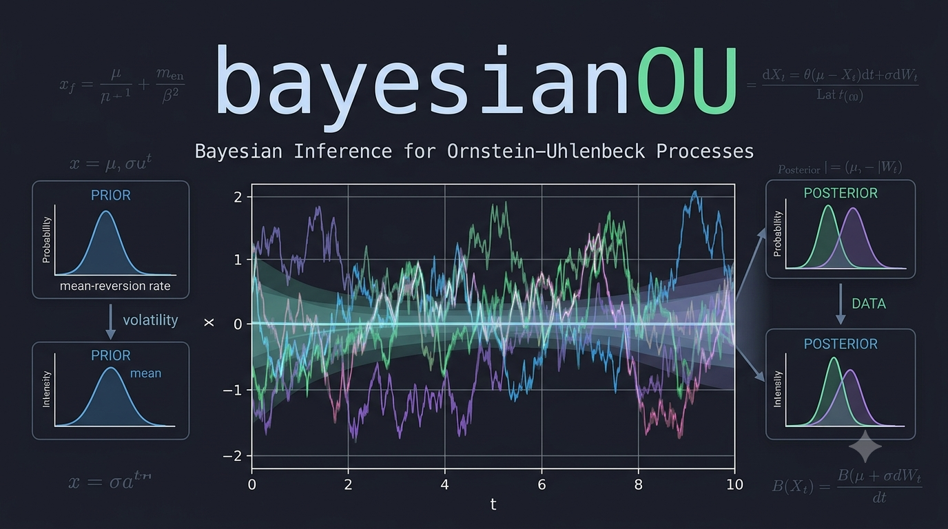
    bayesianOU: Exploring Market Price Gravitation via Ornstein-Uhlenbeck Process

    You can also find this library at CRAN and download it directly from R and RStudio.

    When Market Prices Gravitate: A Bayesian Look at an Old Question in Economics

    An old question, asked again — properly

    There is a question in economics that is older than most of the academic disciplines that border it. Do market prices — the noisy, day-to-day, here-and-now prices at which goods actually change hands — tend to settle toward some underlying center of gravity? And if they do, how fast, how violently, and through what mechanism?

    Classical political economy, from Smith and Ricardo through Marx, thought they do. The idea was that behind the churning surface of market prices there sit “prices of production”: long-run, cost-anchored prices toward which actual prices are pulled, the way a spring pulls a weight back toward its rest position. In the Marxian version, there is one more layer underneath: those prices of production themselves are supposed to gravitate around “values,” the labour embodied in commodities. Whether any of this is true is an empirical question, and for a long time the empirical tools to answer it were not really up to the job.

    A small R package called bayesianOU, written by José Mauricio Gómez Julián and hosted on GitHub, takes a serious swing at that question. It is not the first attempt to test price gravitation statistically, but it is one of the most technically careful I have seen, and it is built in a way that is instructive far beyond the Marxian debate that motivates it. What follows is a walkthrough of what the package does, why it is interesting, and — just as importantly — where it honestly admits its own limits.

    The tool that makes it possible: the Ornstein-Uhlenbeck process

    Strip the economics away for a moment and the statistical core of the package is a workhorse object from physics: the Ornstein-Uhlenbeck (OU) process. Imagine a particle moving in a fluid, attached to a spring. Brownian motion jiggles it randomly; the spring pulls it back toward a fixed point. The further it drifts away, the harder the pull. The result is a wiggly series that never settles but always tends to settle — a mean-reverting random walk.

    The OU process is exactly the mathematical object you want when you suspect a variable is noisy but anchored. It has a “speed of reversion” (how hard the spring pulls) and an “equilibrium level” (where the spring’s rest point is). Estimate those, and you can say something quantitative about gravitation: not just “yes, prices come back,” but “they come back with a half-life of about nine years.”

    That number — the half-life — is the prize. It is the difference between “market prices eventually settle” (which could mean anything) and “market prices settle on a timescale comparable to a business cycle” (which is a falsifiable, interpretable claim).

    What the package actually builds

    The package fits, by Bayesian inference, a family of models built on the OU process but considerably richer than the textbook version. There are two first-class models, sharing one inference engine.

    The single-level model

    The first model asks: do market prices revert toward an equilibrium that is a function of the prices of production, and what does that reversion look like once we let it be nonlinear, volatile, heavy-tailed, and structurally heterogeneous across sectors?

    Each of those adjectives is doing real work, and each corresponds to a feature that simpler approaches handle poorly or not at all:

    • Nonlinear drift. A plain OU process pulls back with a force proportional to the deviation. The package allows a cubic correction, so the restoring force can strengthen super-linearly when prices are far from equilibrium. This matters: real markets may behave gently near the center and violently at the extremes, and a linear model cannot represent that.
    • Stochastic volatility. Financial data, and economic data generally, go through quiet stretches and turbulent ones. The package does not assume a single noise level; it lets the volatility itself wander over time, following its own mean-reverting process on the log-variance. This is the same idea that powers modern stochastic-volatility models in finance, and it is essential for not fooling yourself about the precision of your estimates.
    • Heavy tails. Economic shocks are not Gaussian. Crashes, booms, and policy shocks produce outliers that a normal distribution would call essentially impossible. The package uses Student-t innovations and estimates the degrees of freedom from the data, so the model can discover for itself just how fat-tailed the world is.
    • Hierarchical structure across sectors. An economy has dozens of sectors, and each one presumably has its own reversion speed, its own equilibrium, its own noise. Estimating each sector in isolation throws away the information that they are all part of the same economy. Estimating them all with one set of parameters pretends they are identical. The package takes the middle path — hierarchical, or “partial pooling,” priors — where each sector’s parameters are drawn from a shared distribution whose properties the model also estimates. Sectors borrow strength from one another without being forced into lockstep.
    • A time-varying coupling. This is the most economically loaded feature. The strength with which market prices track prices of production is allowed to depend on the aggregate profit rate (what the package calls TMG). When the general rate of profit is high, the pull of production prices on market prices may be one thing; when it is low, another. Whether that modulation exists, and in which direction, is a hypothesis the model can test rather than assume.

    All of this is estimated jointly, with full Bayesian uncertainty, using Stan’s Hamiltonian Monte Carlo sampler. You do not get a point estimate of the reversion speed; you get a posterior distribution, and from it a credible interval and a probability statement like “there is a 95% chance the half-life is between six and eighteen years.”

    The nested cascade

    The second model is the more ambitious one, and it is where the package earns its “nested” branding. Instead of market prices reverting to a fixed equilibrium, they revert to a latent production price — a hidden, unobserved series that itself evolves over time according to its own OU process, driven by the general profit rate. And, if you turn on the third level, that latent production price in turn gravitates around an observed “value” index built directly from labour-content accounting.

    So the full structure is a cascade: market price → latent production price → value. Each arrow is an OU reversion, each with its own speed, and the speeds are constrained so that the outer (market) layer reverts faster than the inner (production) layer — an economically natural separation of timescales, enforced softly so the data can push back.

    The reason this matters is that it converts a slogan — “prices of production gravitate around values” — into a literal statistical hierarchy that can be fit to data and compared against alternatives. The headline empirical result, from a fit to 37 US sectors over 1960–2020, is a value-coupling coefficient essentially equal to one, with the posterior probability of it being positive effectively equal to one. In plain terms: in standardized units, prices of production track labour values almost one-for-one. That is a found result, not an assumed one — the prior on the coupling was centred at zero, deliberately neutral.

    The inference engine, and why it is not a footnote

    It would be easy to glance at the model description, nod, and move on. But how these quantities are estimated is half of what makes the package serious, and it is worth a paragraph for readers who do not think about MCMC every day.

    Bayesian inference works by exploring the space of all parameter values consistent with both the data and the prior, and characterizing that space as a probability distribution. For models this complex — with latent volatility paths, hierarchical structure, and hundreds of parameters — you cannot do that with pencil and paper. You use a Markov chain Monte Carlo sampler, specifically Hamiltonian Monte Carlo, which borrows an idea from physics: give the parameter space a “potential energy” (the log-posterior) and a “kinetic energy” (a randomly chosen momentum), and let the system glide around the posterior like a ball rolling over a landscape.

    Stan’s NUTS sampler automates this about as well as it can be automated, and the package uses it with within-chain parallelism (via Stan’s reduce_sum) to handle the fact that the likelihood must be summed over many timepoints and sectors. The diagnostics — R-hat for chain agreement, effective sample size, divergence counts — are surfaced through a validate_ou_fit function, and the package is explicit that you should look at them before believing anything.

    Model comparison is done with PSIS-LOO, a clever technique that approximates leave-one-out cross-validation without refitting the model dozens of times, by reweighting the posterior draws using importance sampling. It is the modern standard, and the package is appropriately cautious about it: because the model has a latent volatility state at every observation, plain LOO is known to be optimistic, and the documentation says so plainly.

    The honesty that makes it credible

    Here is where the package surprised me, and here is why I think it deserves a wider audience than the Marxian-economics niche it lives in.

    A naïve reading of the results would be triumphant: the value coupling is one-to-one, the reversion exists, the half-life is about nine years. But the package’s own validation section does something rare. It runs the model against legitimate rivals on genuinely held-out data — a full decade, 2011 to 2020 — and reports, without spin, that a random walk beats the OU model at forecasting, that a no-gravitation restriction ties or beats it, and that the value term adds no detectable predictive density.

    That sounds like a refutation. The package argues, carefully, that it is nothing of the sort — and the argument is the most intellectually interesting thing here.

    The key move is to distinguish two different questions. One is structural: does a reversion mechanism exist, and how fast is it? The other is predictive: can you forecast next year’s price better than a naïve benchmark? These are related but not identical, and for a slow process they come apart in a specific, predictable way.

    If gravitation is real but slow — a half-life of nine years on a dataset whose test window is a decade — then over the forecast horizon the process looks, to first order, like a random walk. The reversion is there, but it is too weak to show up in a one-step or few-step prediction. The random walk, which assumes no reversion, will forecast almost as well, because over short horizons a barely-reverting process and a non-reverting one are nearly indistinguishable. So the random walk winning the forecasting horse race is not evidence against gravitation; it is evidence consistent with gravitation being slow.

    This is not special pleading. It is a logical point about what different functionals of a model can and cannot tell you. The structural parameters — estimated from the joint likelihood over the whole panel, borrowing strength across 37 sectors and 61 years — use far more information than any single-series forecast. They can pin down a central tendency that a univariate test cannot. And the package shows, through simulation-based calibration and adversarial negative controls, that the estimation pipeline does not manufacture gravitation when none is present: feed it a true random walk and it reports a half-life of about fifty years; feed it a null value-coupling and the posterior honestly covers zero.

    The low-kappa trap, and why it matters to everyone

    The package names a difficulty it calls the low-kappa trap, and it is worth understanding because it is a trap that catches far more than Marxian price theory.

    Kappa is the reversion speed. As kappa shrinks toward zero, the OU process approaches a pure random walk. The trouble is that there is no bright line separating “slow mean reversion” from “no mean reversion.” It is a continuum, and three distinct problems stack up exactly there:

    • Algebraically, reversion speed and discrete-time persistence are two sides of the same coin; kappa going to zero is the same as the autocorrelation going to one. There is no internal frontier.
    • Statistically, the power of a unit-root test — the standard tool for asking “is this a random walk?” — collapses exactly as the truth approaches the random walk boundary. With a finite sample and a half-life comparable to the sample length, the test simply cannot tell. This is a well-known result in econometrics, and it is why decades of “is the real exchange rate stationary?” papers argued past one another.
    • Numerically, if the reversion speed is parameterized to be strictly positive (as it must be, for the sampler to behave), then “the probability that kappa is greater than zero” is trivially one — it tells you nothing. The informative quantity is the half-life, and the probability that the half-life exceeds some sensible horizon.

    The package’s response to the trap is instructive. It does not pretend the trap is not there. It states all three layers explicitly, reports the slow tail honestly (one sector has a non-trivial posterior probability of a half-life beyond forty years), and argues that the joint hierarchical posterior — which pools information across the whole panel — is a more powerful discriminator than any univariate test. That is a defensible position, and it is stated with the caveat attached rather than buried in a footnote.

    This is the broader lesson. Anyone working with time series that might be slowly mean-reverting — interest rates, real exchange rates, commodity prices, climate variables, pollutant concentrations — runs into exactly this trap. The package’s framing of it, in three layers, is one of the clearest expositions I have read, and it would travel well into any of those domains.

    What I appreciate, and what I would watch for

    A few things stand out as genuinely good practice, and they are worth naming because they are rarer than they should be.

    The separation of economic and sampler convergence. The package is scrupulous about not confusing two senses of “convergence.” Economic convergence — does the price revert? — is a statement about kappa and the half-life. Sampler convergence — did the MCMC chains agree? — is a statement about R-hat and divergences. These share a word and nothing else, and conflating them is a classic source of muddled reasoning. The documentation keeps them lexically distinct throughout.

    Neutral priors on the load-bearing hypotheses. The prior on the profit-rate modulation is centred at zero. The prior on the value coupling is centred at zero. The package does not bake the answer into the question. When the posterior then moves clearly away from zero, that means something.

    Out-of-sample integrity by construction. A subtle and common error in time-series work is “leakage”: accidentally letting future information contaminate the training procedure, so that out-of-sample results are secretly in-sample. The package offers a fit_window switch that keeps the two designs genuinely separate, and it computes the common-factor loadings from the training window only. This is the kind of plumbing detail that separates trustworthy work from work that just looks trustworthy.

    The negative results are reported. Many packages, and most blog posts about them, would quietly omit the fact that a random walk out-forecasts the model. This one leads with it and then reasons about it. That is how a field accumulates reliable knowledge rather than just encouraging headlines.

    What should a careful reader watch for? The half-life estimate of about nine years is, by the package’s own account, probably conservatively slow — a controlled study of the disaggregation step suggests the true figure may be closer to seven or eight. The cubic nonlinearity is a minor refinement on this data (its coefficient sits near its prior). The Student-t degrees of freedom and the stochastic-volatility scale are weakly identified when both are present, a known tension the documentation flags but does not resolve. And the headline value-coupling result, while striking, is measured on standardized levels that share a cost-price component by construction; the package defends this with a “wedge” argument — subtracting the shared component and testing the residual — but a sceptical reader should follow that argument itself rather than take it on trust.

    None of these caveats undermine the project. They are the project. A statistical framework that cannot articulate its own soft spots is not a framework you should believe.

    Why it is worth your time

    You do not need to be a Marxian economist, or any kind of economist, to get something out of this package. If you work with time series that exhibit slow, noisy reversion toward a moving target — and a great deal of the physical and social world does — the modelling ideas here are directly portable: the nonlinear OU drift, the stochastic volatility, the hierarchical pooling across groups, the careful separation of structural estimation from forecasting, and the three-layer diagnosis of the low-reversion trap.

    And if you are interested in the classical question of whether prices gravitate toward values, this is about as good a statistical treatment as you will find: modern machinery, honest reporting, and a willingness to let the data argue back against the theory that motivated the exercise in the first place.

    The repository, the full mathematical specification, the validation blocks, and a frank discussion of every methodological decision live at github.com/IsadoreNabi/bayesianOU, with the wiki carrying the complete technical detail. Read the methodology notes before you quote a number; that is what they are there for.

  • Quantitative Theory of Money or Prices? A Historical, Theoretical, and Econometric Analysis

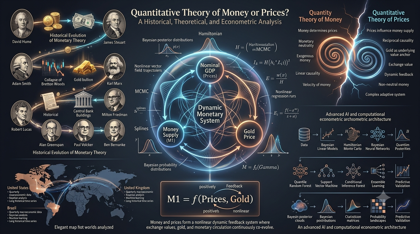
    Quantitative Theory of Money or Prices? A Historical, Theoretical, and Econometric Analysis

    Does Money Drive Prices, or Do Prices Drive Money?
    Econometrics · Monetary Theory · Machine Learning · Political Economy

    Does Money Drive Prices, or Do Prices Drive Money?

    A 300-year-old debate, four countries, six decades of data, Bayesian statistics, and neural networks — a deep dive into one of the most ambitious monetary studies in recent years

    What you will find in this post
    1. The oldest argument in monetary economics — Hume, Friedman, and why it still matters today
    2. Marx’s forgotten critique — four logical objections that mainstream economics never answered
    3. The role of gold in a post-gold-standard world — why the Fed still dances around the price of gold
    4. A mathematical model for the money-prices relationship — equations explained without the jargon
    5. The data and the methodology — four countries, Bayesian models, neural networks, and random forests
    6. Country-by-country results — what the United States, Canada, the UK, and Brazil each reveal
    7. Why money is never neutral — and what that means for how we think about the economy
    8. Policy implications and open questions — what this means for central banks and for you
    · · ·

    1. The Oldest Argument in Monetary Economics

    There is a question at the heart of economics that sounds deceptively simple: when governments print more money, do prices go up because there is more money chasing the same goods — or does the economy first produce goods at certain prices, and then the amount of money in circulation simply adjusts to match? Put differently: does money cause prices, or do prices cause money?

    This is not an abstract riddle for seminar rooms. The answer determines how central banks set interest rates, whether governments choose austerity or stimulus in a recession, and how we understand inflation. If the quantity of money determines prices, then controlling the money supply is the key to controlling the economy. If prices determine the quantity of money, then the real action is in production, technology, and competition — and monetary policy is, at best, a secondary lever.

    The debate begins with the Scottish philosopher David Hume, writing in the mid-eighteenth century. In his essays on money and trade, Hume proposed what became the foundation of mainstream monetary thought: if you double the quantity of money in an economy while keeping everything else constant, prices will eventually double. Money, in this view, is a veil — it changes the numbers on price tags but does not alter the real productive capacity of the economy. The ratio of money to goods simply adjusts until equilibrium is restored.

    This idea was not without immediate critics. The Scottish economist James Steuart attacked it almost as soon as it appeared (1767). Adam Smith, often considered the father of modern economics, held the opposite view — that prices, not money, are the active variable. But the idea proved remarkably resilient. Over the following two centuries, it was refined into what economists call the Quantity Theory of Money, which reached its most influential modern form in the work of Milton Friedman. For Friedman, Hume was the starting point of all monetary theory. For Robert Lucas, another Nobel laureate, Hume marked the beginning of modern monetary economics.

    But there was always an alternative tradition, running from the classical economists through Karl Marx, that saw the relationship in exactly the opposite direction. A new paper by the Costa Rican economist José Mauricio Gómez Julián, published on arXiv in January 2025, takes this alternative tradition seriously, subjects it to rigorous empirical testing with the most modern tools available — Bayesian statistics, machine learning, deep learning, and ensemble methods — and arrives at conclusions that challenge the mainstream consensus.

    · · ·

    2. Marx’s Forgotten Critique

    When most people hear “Marx” and “money” in the same sentence, they expect ideology. But in his Contribution to the Critique of Political Economy (1859), Marx offered something far more valuable: a meticulous logical dissection of Hume’s reasoning. Gómez Julián’s paper draws on four central aspects of this critique, each of which makes testable claims about the real world.

    First: Money is subordinated to exchange values, not the other way around

    Marx’s fundamental point is that the sphere of circulation (where money changes hands) is ultimately subordinated to the sphere of production (where goods are actually made). This is not just a philosophical claim — it has a concrete implication. The quantity of money in circulation must maintain a certain equilibrium with the quantity of goods and services available for sale. If there is too little money, commercial transactions become difficult — there are not enough means of payment to go around. If there is too much money, sellers can raise prices to absorb the excess.

    But here is the crucial mechanism: if the quantity of money falls below or rises above its “necessary level,” a coercive correction occurs through commodity prices. Prices adjust, and money supply follows — not the other way around. The direction of causation runs from prices to money, mediated by the real commodity foundation of money (in Hume’s and Marx’s time, gold and silver).

    This means that money’s non-neutrality — the fact that changes in the money supply do affect real economic outcomes — is not caused by money determining prices. It is caused by the mediating relationship between prices and the material foundation of money, which creates a feedback loop over time.

    Second: An epistemological critique of Hume’s evidence

    Marx points out that when Hume formulated his theory, he was observing a very specific historical situation: the discovery of American mines and the increase in slave labor, which lowered the extraction cost of gold and silver. Under these conditions, the price of commodities exchanged directly for gold and silver (i.e., exported commodities) did indeed rise. But this rise occurred because gold and silver were functioning as commodities — their production cost had dropped — not because more money was chasing the same goods. The effect on gold as a means of payment (i.e., domestic money) took much longer to materialize. Hume, in Marx’s reading, confused a change in the relative value of a commodity (gold) with a general monetary phenomenon.

    Third: Accounting money vs. means of circulation

    Marx argues that Hume made a fundamental category error: he confused accounting money (the unit in which prices are denominated) with money as a means of circulation (the physical medium of exchange). These are different things with different behaviors. Moreover, Hume failed to consider historical events of his own time that demonstrated the need to account for the exchange value of gold and silver when linking money to prices.

    Fourth: Two critical corollaries

    This is where the theory makes its sharpest predictions. Marx draws two conclusions from his analysis that can be tested empirically:

    Marx’s two testable corollaries
    • Corollary 1: If metallic currency is a symbol of value, then the sum of commodity prices determines the quantity of circulating money. But if the monetary unit is a symbol of value, then the quantity of circulating money is determined by the sum of commodity prices. Marx argues it is the monetary unit — not the metallic currency — that is the symbol of value.
    • Corollary 2: If money derives its value from prices (Marx’s position), then there can be more money in circulation than the sum of commodity prices. But if money determines prices (Hume’s position), then there cannot be more money circulating than the sum of prices. Marx argues that the former is true — and it can be checked against data.

    Gómez Julián checks Corollary 2 directly. “Circulating money” is defined as the monetary aggregate M1 (cash plus checking deposits), and the “sum of commodity prices” is, by definition, nominal GDP. Looking at the statistical systems of the United States, the United Kingdom, Canada, and Brazil, the paper finds that M1 exceeds nominal GDP in multiple years for each country. This is straightforward evidence in favor of Marx’s position. The author also notes that previous work on El Salvador showed M1 consistently below nominal GDP — which might seem to contradict the pattern until one considers El Salvador’s dollarization, which fundamentally changes the monetary dynamics.

    “Marx’s central thesis is that the value of money depends on the purchasing power of the commodity or commodities that underlie it, and this purchasing power, in turn, depends on the general level of prices. Such prices, the market prices, are determined by capitalist competition.” — Gómez Julián, summarizing Marx’s framework

    The value theory question

    One cannot discuss Marx’s monetary theory without addressing the foundation beneath it: the labor theory of value (LTV). Marx argues that market prices oscillate around “prices of production,” which are themselves grounded in the socially necessary labor time required to produce goods. If the LTV is correct, then exchange values have an objective basis in production — and the subordination of money to prices follows naturally.

    The paper acknowledges that these monetary claims stand or fall with the validity of the LTV, but it also notes that the neoclassical alternative — the subjective theory of value based on marginal utility — has its own deep problems. The famous Cambridge Capital Controversy of the 1960s demonstrated that the neoclassical foundations (the so-called “neoclassical parables”) do not provide a coherent scientific explanation of economic phenomena. Even Paul Samuelson, one of the greatest neoclassical economists, admitted that capital aggregation problems can only be resolved by adopting something very close to the labor theory of value. Joan Robinson went further, arguing that capital can be nothing more than “accumulated past labor.” Notably, the Penn World Tables — one of the most important databases in empirical economics — do not use marginal productivity of capital to measure capital remuneration, but instead use the real average internal rate of return, precisely because of the aggregation problem.

    · · ·

    3. The Role of Gold in a Post-Gold-Standard World

    If money is ultimately subordinated to prices, and prices are anchored in the real economy, what gives money its value in the modern era? Since the collapse of the Bretton Woods system in 1971, when President Nixon ended the dollar’s convertibility to gold, most economists have treated modern money as purely “fiduciary” — backed by nothing but government decree and public trust. Gómez Julián argues, with substantial evidence, that this is not the full picture.

    The paper presents three pillars of evidence for gold’s continuing monetary role:

    Gold’s enduring monetary significance
    • Greenspan’s own words: “Gold still represents the ultimate form of payment in the world. Fiat money in extremis is accepted by nobody. Gold is always accepted.” This is not a gold bug’s fantasy — it was stated by the man who chaired the Federal Reserve for nearly two decades.
    • The inverse relationship: Gold and the US dollar consistently move in opposite directions. When gold rises, the dollar tends to fall, and vice versa. This has been documented by multiple financial analysts and is visible in decades of market data.
    • Policy history: After the turbulence of the 1970s (high inflation, debt crises, savings crises), Paul Volcker — who took over as Fed chair in 1979 — formally abandoned the monetarist experiment in 1982 and adopted policies aimed at stabilizing the dollar’s value against gold and other commodities. This was supported by the Plaza Accord (1985) and the Louvre Accord (1987). The result was the “Great Moderation” (1982–2007), a period of unusual macroeconomic stability.

    The paper traces a revealing pattern through subsequent Fed chairs. Greenspan continued Volcker’s gold-aware approach. When Ben Bernanke — an economist who openly declared Friedman as his central intellectual influence — took over in 2006, policies diverged from the gold anchor, and gold price volatility surged to its highest level since the end of Bretton Woods. The dollar declined. Janet Yellen, who succeeded Bernanke in 2014, returned to the Volcker-Greenspan orientation, and gold prices stabilized. Jerome Powell initially followed this path but gradually moved away, declaring in 2019 that tying the dollar to gold would prevent the Fed from maximizing employment.

    Gómez Julián pushes back on Powell’s argument on two grounds. First, periods when the Fed stabilized the dollar around gold showed at least the same level of employment stability as periods when it did not. Second, since Bretton Woods, no country has used the gold standard directly — they have anchored their currencies to the dollar, and the dollar has been anchored (in varying degrees) to gold. So Powell’s claim that “no country uses it” misses the layered structure of the international monetary system.

    The dialectical contradiction of gold

    The paper draws on the Marxist economist Ernest Mandel to explain why the United States both needs and resists the gold standard. The gold standard provides stability — but it also requires contractionary policies during recessions, which can deepen crises and, as the case of Heinrich Brüning’s Germany (1930–1932) showed, can undermine democracy by creating the conditions for fascism. The gold standard also requires a delicate balance between short-term dollar demand (from foreign investors parking reserves) and long-term dollar outflow (from American investments abroad). When this balance tips — as it did in the late 1960s — the result is a monetary crisis.

    “The ‘dollar crisis’ and the search for means of international payment independent both of gold and ‘currency reserves’ reflect clear recognition on the part of big international capital of a contradiction inherent in the present-day capitalist system: the contradiction between the dollar’s role as an ‘international money,’ and its role as an instrument to assure the expansion of the American capitalist economy. To fulfill the first function, a stable money is needed. To fulfill the second function, a flexible money is necessary, i.e., an unstable one. There’s the rub.” — Ernest Mandel, 1968, quoted in the paper

    This dialectical tension — the system needs gold stability but also needs monetary flexibility — explains the recurring oscillation between gold-anchored and gold-detached monetary regimes. The paper describes the current arrangement as a “loose gold standard”: not a formal peg, but a persistent gravitational pull.

    · · ·

    4. A Mathematical Model for the Money-Prices-Gold Relationship

    Gómez Julián formalizes the above arguments into a mathematical model. The basic version is elegant in its simplicity:

    Core equation Qm = λp / λgold · β

    In plain language: the quantity of money in circulation (Qm, measured as M1) is equal to the sum of commodity prices (λp, measured as nominal GDP) divided by the international price of gold (λgold), multiplied by a coefficient (β) that represents the velocity of money circulation (assumed, for simplicity, to equal one).

    This equation encodes several intuitive relationships:

    What the equation says — in words
    • If prices (nominal GDP) rise while gold stays the same, the money supply must increase — more money is needed to express the same goods at higher prices.
    • If the gold price rises while prices stay the same, the money supply decreases — fewer monetary units are needed to express the same sum of prices, because gold is now more valuable per unit.
    • If both prices and gold rise, the effect on money depends on which change is larger — it could go either way.
    • If prices rise and gold falls, money unambiguously increases — both forces push in the same direction.

    The paper works through all eight possible combinations of price and gold movements (both up, both down, one up one down, one fixed one moving, etc.), showing that the model’s predictions are internally consistent. This is not just algebra — it is a stress test of the theory’s logical coherence.

    The model can also be expressed in logarithmic form, which has a practical advantage: when you run a regression on logarithmically transformed variables, the coefficients can be interpreted directly as elasticities — percentage changes. For example, a coefficient of 0.13 means that a 1% increase in prices is associated with a 0.13% increase in the money supply, holding gold constant. This logarithmic transformation also tends to smooth out extreme values in the data, improving statistical performance.

    A more general version of the model simply states that the money supply is a function of both prices and gold, without specifying the exact functional form — leaving the data to reveal the shape of the relationship.

    · · ·

    5. The Data and the Methodology

    Four countries, carefully chosen

    The empirical analysis covers quarterly data from four countries, each chosen for a specific reason:

    Country selection and rationale
    • United States (1959–2022): The most developed Western capitalist economy. Economic laws derived from its study are, to varying degrees, applicable to other capitalist countries. It represents the highest stage of development reached by Western capitalism and serves as a mirror of the future for other economies. 63 years of data — longer than a Kondratieff wave (the long cycles of capitalist dynamics, typically 40–60 years).
    • Canada (1961–2022): Chosen for similar reasons to the UK, but representing the welfare state variant of Western capitalism — a different model from both the US and the UK. 61 years of data.
    • United Kingdom (1986–2022): A major developed capitalist economy with more available data than other candidates like Germany or France. 36 years of data.
    • Brazil (1996–2022): An emerging economy (developing country), chosen to test whether the findings generalize beyond advanced capitalism. Since the study had already been done for El Salvador (an underdeveloped country), verifying the results for Brazil would suggest the patterns are general economic laws of capitalist development. 26 years of data.

    A multi-layered methodological approach

    This is not a paper that runs one regression and calls it a day. The methodology unfolds in several stages, each building on the previous one:

    Stage 1: Pairwise direction analysis. The first question is: for each pair of variables (money-prices, gold-prices, money-gold), which variable best predicts which? This is done using Bayesian simple linear regression, where the direction of the relationship is determined by comparing the Expected Log Pointwise Predictive Density from Leave-One-Out cross-validation (ELPD-LOO) — a rigorous measure of how well a model predicts data it has not seen. Higher (less negative) ELPD-LOO means better predictive performance.

    Stage 2: RESET tests for nonlinearity. Linear models assume straight-line relationships. But what if the real relationship is curved? The paper runs Ramsey’s RESET test with quadratic, cubic, and combined terms, bootstrapped using a Bayesian posterior distribution. This reveals whether linear models are missing important nonlinear patterns — and, if so, what kind of curvature is present.

    Stage 3: Empirical distribution fitting. Before building multivariate models, the paper determines the best-fitting probability distribution for each variable (log-normal, Weibull, Gamma, Normal, etc.) using the maximum goodness-of-fit method, with results selected by the Bayesian Information Criterion (BIC). This is not just a technical exercise — it directly informs how the variables are transformed in later models.

    Stage 4: Bayesian Generalized Linear Models (BGLM). The paper constructs multivariate models using different statistical families (Gamma, Gaussian) and link functions (logarithmic, identity), with gold often transformed into a natural cubic spline (a flexible curve that can capture nonlinear patterns) or fitted as a Weibull random variable. The choice of family, link, and transformation is driven by predictive performance metrics.

    Stage 5: Machine learning and deep learning. Four different ML models are tested individually and in combination:

    Machine learning models used
    • Quantile Random Forest (QRF): An extension of random forests that estimates the entire distribution of the predicted variable, not just its average.
    • Conditional Inference Random Forest: A variant that uses statistical tests to select splitting variables, reducing bias toward variables with many possible splits.
    • Bayesian Regularized Neural Network (BRNN): A neural network that uses Bayesian regularization to prevent overfitting — the model learns to be cautious about its own complexity.
    • Support Vector Machine with Radial Basis Kernel (SVMRadial): A powerful classification/regression method that maps data into higher-dimensional spaces to find optimal decision boundaries.

    Stage 6: Ensemble learning. Finally, the paper tests whether combining multiple models through boosting (a technique where each new model focuses on the errors of the previous ones) produces better predictions than any individual model. The ensemble is structured as a Bayesian Generalized Linear Model with Gaussian family and identity link.

    A critical philosophical point: the paper uses objective Bayesian analysis. This means that all prior information — the starting assumptions the model uses before seeing the data — is derived from empirical analysis of the dataset itself, not from subjective beliefs or assumptions. This approach incorporates what the author calls “epistemological doubt” about parameter estimation, acknowledging that we can never be perfectly certain about any estimated value.

    · · ·

    6. Country-by-Country Results

    United States (1959–2022)

    The pairwise analysis reveals something striking: the simple relationship between M1 and prices is undecidable — both directions fit about equally well by ELPD-LOO. This is already a blow to the simplistic Quantity Theory, which claims a clear causal arrow from money to prices. However, gold is clearly best predicted by prices (not the reverse), and M1 is clearly best predicted by gold (not the reverse). This suggests a chain: prices → gold → money, consistent with Marx’s framework.

    The RESET tests confirm that the relationships are nonlinear. For the M1-prices pair in both directions, all RESET tests yield p-values of zero — meaning the linear models are definitively inadequate. Nonlinearity is everywhere.

    The multivariate model that best fits the data is a BGLM with Gamma family, logarithmic link, and gold transformed into a natural cubic spline with five degrees of freedom. The coefficient on log(prices) is +0.13 — confirming the direct, positive relationship between prices and money supply. The spline coefficients for gold alternate in sign across the five basis functions, confirming the theoretically predicted nonlinear, segment-dependent relationship. The model achieves an MAE of just 0.12 (2.43% of the log(M1) minimum) and an RMSE of 0.21.

    The ensemble model — combining a Bayesian Regularized Neural Network (weight: 0.41) and a Quantile Random Forest (weight: 0.59) — further improves performance: MAE drops to 0.08 on test data, RMSE to 0.25, and the R² reaches 0.985 in training. All coefficients are highly significant (p < 2e-16). The US is the only country where the ensemble outperforms the best individual ML model.

    Canada (1961–2022)

    The pairwise results are cleaner than in the US case: M1 is best predicted by prices, gold is best predicted by prices, and M1 is best predicted by gold. The chain prices → gold → money is clearly visible. RESET tests again confirm pervasive nonlinearity.

    The best multivariate model uses a BGLM with Gamma family, logarithmic link, and gold transformed as a Weibull random variable (shape = 5.88, scale = 6.47). The coefficient on log(prices) is +0.045 — smaller than in the US but still positive and confirming the prices-to-money direction. The Weibull transformation captures the nonlinear gold dynamics in a single parametric term. The model achieves an MAE of 0.23 and RMSE of 0.28.

    Unlike the US, the ensemble did not improve on the best individual ML model. A Quantile Random Forest performed best on its own, achieving a remarkable R² of 0.998 in training and an MAE of just 0.04 on test data. The near-perfect fit suggests that the money-prices-gold relationship in Canada is highly regular and predictable over this period.

    United Kingdom (1986–2022)

    With a shorter sample (36 years), the UK shows a more mixed pattern in pairwise analysis. Notably, the simple relationship between M1 and prices runs in the reverse direction — prices are best predicted by M1, not the other way around. This might seem to support the Quantity Theory, but it only holds in the simple bivariate case. When gold is included in the multivariate model, the direct relationship between prices and money reasserts itself.

    The best multivariate model is a BGLM with Gamma family, logarithmic link, and gold transformed as a natural cubic spline with five degrees of freedom — similar to the US specification. The coefficient on log(prices) is +0.071, and the spline coefficients alternate in sign, as predicted by theory. The model achieves an MAE of 0.06 and RMSE of 0.07 — the tightest fit among the four countries.

    As with Canada, the ensemble did not improve on the best individual model. A Quantile Random Forest again performed best, with R² of 0.993 in training and near-zero RMSE on test data.

    Brazil (1996–2022)

    Brazil, as an emerging economy with a turbulent monetary history, presents the most complex picture. In pairwise analysis, the money-prices relationship again runs in the reverse direction (prices predicted by M1), and the gold-prices relationship is bidirectional. RESET tests show the strongest nonlinearity signals of any country, with many p-values at or near zero.

    The best multivariate model uses a BGLM with Gaussian family (the only country where Gaussian outperformed Gamma), logarithmic link, and gold transformed as a natural cubic spline. The coefficient on log(prices) is +0.05, again confirming the direct relationship. Model performance is solid: MAE of 0.07, RMSE of 0.21.

    Among ML models, a Support Vector Machine with Radial Basis Kernel performed best, achieving R² of 0.991 in training and an MAE of 0.012 on test data. As with Canada and the UK, the ensemble did not improve on this individual model.

    Summary: In all four countries, the multivariate models confirm a positive relationship between prices and money supply, and a nonlinear, segment-dependent relationship between gold and money supply — exactly as the theoretical model predicts.
    · · ·

    7. Why Money Is Never Neutral

    The paper’s central conclusion, stated plainly: money is not neutral at any time horizon — not in the short run, not in the long run, across all four countries studied.

    This is a strong claim, and it contradicts one of the most fundamental assumptions of mainstream economics. The concept of “monetary neutrality” holds that changes in the money supply eventually affect only nominal variables (prices, wages) and leave real variables (output, employment) unchanged. In the long run, the argument goes, the economy returns to its “natural” state regardless of what the central bank does with the money supply.

    Gómez Julián’s results, based on data spanning up to 63 years — longer than a full Kondratieff cycle — provide no support for this proposition. But the paper is careful to explain why money is non-neutral, and the explanation differs from what both mainstream and some heterodox economists might expect.

    Non-neutrality, in this framework, is not caused by the money supply determining prices (the monetarist claim). It is caused by the mediating relationship between prices and the real commodity foundation of money (gold), which determines the money supply. This creates a feedback loop: prices influence gold, gold influences money, and money — through aggregate demand — feeds back into prices. The exchange value of money as a monetary unit is the transmission mechanism.

    Because this feedback is nonlinear (as confirmed by the RESET tests and the spline models across all four countries), and because it operates over time with dynamic lags, the money-prices-gold system constitutes what complexity scientists would call a complex system — a system where small changes can have disproportionate effects, where cause and effect are intertwined, and where linear prediction is fundamentally limited.

    · · ·

    8. Policy Implications and Open Questions

    What this means for policy

    The findings have practical consequences for how we think about monetary policy:

    Policy takeaways
    • The best way to control prices is directly — through industrial policy, competition policy, supply-side interventions, and measures that address the real determinants of production costs. Since prices are ultimately grounded in the sphere of production, intervening there is the most effective approach.
    • But controlling the money supply also works — because the feedback relationship runs in both directions. Contracting M1 can reduce prices, even though the primary direction of causation runs from prices to money. This “theoretically justifies a commonly effective practice in economic policy,” as the author puts it.
    • Friedman’s narrative about the Great Depression is weakened. The Federal Reserve expanded the monetary base during the Depression, yet the Depression happened anyway. During the 2008 crisis, the Fed adopted an aggressive expansionary monetary policy — and it alone was not enough. It had to be accompanied by massive fiscal intervention (the 2009 American Recovery and Reinvestment Act), direct asset purchases, near-zero interest rates, and other measures. As Krugman noted, “The Monetary History thesis has just taken a hit.”
    • The gold standard is not incompatible with employment stability. This challenges the argument, made by Jerome Powell and others, that returning to a gold anchor would sacrifice the Fed’s ability to maximize employment. The historical record shows at least equivalent macroeconomic stability during gold-anchored periods.

    Two open questions for future research

    The paper is transparent about what it does not answer:

    Question 1: In the current loose gold standard, how exactly does the feedback between prices, gold, and the money supply work through specific economic policy instruments? The Fed’s tools — interest rates, quantitative easing, reserve requirements — act as latent variables mediating the gold-money relationship. The paper establishes that this mediation exists but acknowledges that its precise mechanisms require further study.

    Question 2: What are the quantitative and temporal limits of monetary non-neutrality? If too much money enters circulation, commodity prices eventually correct the imbalance through a “coercive correction.” But how large can the distortions become before correction occurs, and how long does the adjustment take? Understanding these limits could illuminate phenomena traditionally attributed to monetary factors — such as the “liquidity trap” — from an entirely new angle.

    A methodological statement

    Beyond its economic findings, the paper is also an argument about method. By combining objective Bayesian statistics with modern machine learning — neural networks, random forests, support vector machines, and boosted ensembles — Gómez Julián demonstrates that the tools of artificial intelligence can serve heterodox economic theory, not just mainstream modeling. Using Bayesian regularized neural networks and gradient-boosted ensembles to test predictions derived from Marx’s nineteenth-century monetary theory is, to put it mildly, unusual. But the results are robust, the fit is strong, and the patterns are consistent across four countries with very different economic structures.

    The paper’s approach to the so-called “transformation problem” — the long-standing debate about how labor values map onto market prices — also deserves attention. By assuming inventory valuation at the cost of reproduction (where the current technological state determines the value of inputs), Gómez Julián shows that the system of equations has a unique solution given the degree of exploitation of labor power, sidestepping a controversy that has occupied Marxist economists for over a century.

    · · ·

    The Takeaway

    Three hundred years after David Hume proposed that money determines prices, and one hundred and sixty-five years after Karl Marx argued the opposite, we still do not have a settled answer. Gómez Julián’s paper does not claim to settle it — but it does something arguably more valuable. It shows, with rigorous data and modern methods across four countries and six decades, that the question itself may be wrongly framed as a binary choice.

    Money and prices, along with gold, form a complex, nonlinear, feedback-driven system in which both directions of causation operate simultaneously. But the relationship is asymmetric: prices hold the upper hand. Money is ultimately subordinated to the real economy — to production, to labor, to the commodities that give currency its value — even as it feeds back into prices through aggregate demand. Money is never neutral, but it is never the master either. It is, in the deepest sense, a dependent variable that nonetheless shapes the system it depends on.

    In an era of quantitative easing debates, cryptocurrency experiments, inflation anxiety, and questions about the very nature of money, this is not just an academic finding. It is a framework for thinking about the monetary world we actually inhabit — one that is messier, more dynamic, and more deeply rooted in material reality than either Hume or Friedman imagined.