Fiscal and Monetary Policy Usually Hold Hands
What 60 years of U.S. data reveal about the myth of independent economic instruments
Imagine you are steering a ship with two sets of controls—one for the rudder and one for the engine. Conventional wisdom says these controls work independently: you can adjust the rudder without affecting the engine, and vice versa. For more than seventy years, this is essentially how mainstream economics has treated a country’s fiscal policy (government spending and lending) and its monetary policy (interest rates and central bank operations). Each set of tools was supposed to be independent of the other, allowing policymakers to pursue multiple goals at the same time without interference.
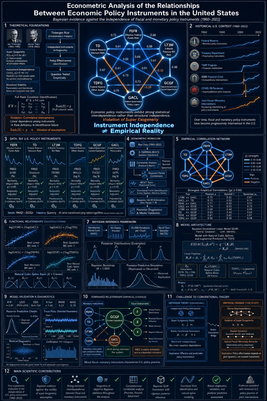
A new study published in the Revista Cubana de Economía Internacional challenges that assumption head-on. Using six decades of quarterly U.S. data—from January 1960 to October 2022—and a battery of modern Bayesian statistical techniques, economist José Mauricio Gómez Julián finds that American fiscal and monetary instruments are far from independent. They are, in fact, deeply intertwined, both in straightforward linear ways and in more complex, nonlinear patterns. The implications ripple outward from econometric theory into the practical world of how governments manage economies.
The Rule That Started It All
The story begins in 1952, when the Dutch economist Jan Tinbergen—who would later share the first Nobel Memorial Prize in Economic Sciences—formulated a deceptively simple principle: to achieve n independent policy goals, you need at least n independent policy instruments. Known today as the “Tinbergen Rule,” this idea became a cornerstone of economic policy theory. It told governments that if they wanted to control inflation, unemployment, and growth simultaneously, they needed at least three tools that did not overlap in their effects.
The American economist James Tobin later sharpened this: instruments are independent when “the effects of any instrument on the targets are not proportional to those of any other, or of any combination of others.” In modern econometrics, this independence assumption has been formalized as super exogeneity—a technical condition saying that the statistical relationships between economic variables remain stable even when policymakers intervene. If super exogeneity holds, a central bank can freely adjust interest rates without worrying that the Treasury’s spending decisions will systematically interfere with those adjustments.
“If a central bank is free to choose the adjustments to its instruments to pursue its final objectives, it has instrument independence.”
— Laurence H. Meyer, former Federal Reserve GovernorThe problem? Despite its foundational role in economic theory, nobody had rigorously tested this assumption econometrically for the U.S. case—until now.
Six Instruments, Six Decades
The study examines six economic policy instruments, divided into two groups:
Instruments Studied
- Fiscal instruments: Federal government current spending (GCGF) and federal government policy lending (GACL)
- Monetary instruments: The effective federal funds rate (FEFR), the Federal Reserve discount rate (TD), other assets held by the monetary authority (TDFG), and the 3-month Treasury bill secondary market rate (LT3M)
Data sourced from the Federal Reserve Economic Data (FRED) database and YCharts, spanning 252 quarterly observations.
With these variables in hand, the researcher embarked on a two-stage investigation. First, he tested whether each pair of instruments showed any meaningful statistical association. Then, he built a predictive model to see whether one instrument could be reliably forecasted from the others—which would be impossible if they were truly independent.
Stage One: Mapping the Web of Connections
The preliminary analysis used three different correlation measures—Pearson, Kendall, and Spearman—in both their classical (frequentist) and Bayesian versions. The results were striking. Eight pairs of instruments showed significant correlations, with partial correlation coefficients at or above 0.5 in absolute value. For context, a Pearson correlation of 0.5 means one variable explains about 25% of the variation in another—a substantial relationship by any standard.
Some highlights from the correlation analysis:
- The 3-month Treasury bill rate and federal policy lending showed a strong positive correlation (Pearson partial correlation of approximately 0.78).
- Federal policy lending and the discount rate were also strongly positively correlated (about 0.77).
- Federal government spending and federal policy lending were negatively correlated (about −0.69), suggesting that as one rises, the other tends to fall.
- Government spending showed negative correlations with all three monetary interest rate instruments (around −0.59 to −0.61).
The fact that these correlations held across different statistical measures and survived the stationarity adjustments (seasonal corrections applied via the X-13ARIMA-SEATS method) gives them added credibility. The seasonality adjustments also provided strong evidence that the variables follow approximately normal distributions, further validating the correlation analysis.
Linearity, Quadratics, and Beyond
Correlation tells you that two variables move together, but not how they move together. Is the relationship a straight line? A curve? Something more exotic? To answer this, the study employed Bayesian linear regression models and RESET tests (a standard diagnostic for detecting nonlinear relationships), both reinforced with Bayesian bootstrapping—a resampling technique that generates thousands of synthetic datasets to test the robustness of results.
The findings revealed that most instrument pairs have linear relationships, but in two notable cases—the discount rate versus policy lending, and the federal funds rate versus government spending—quadratic (curved) relationships also play a role. This means the effect of one instrument on another is not constant; it changes depending on the level of the variable, adding a layer of complexity that the Tinbergen framework simply does not account for.
For example, the relationship between the federal funds rate and government spending follows a parabolic pattern: at lower spending levels, the federal funds rate behaves one way, and at higher spending levels, it behaves differently. This kind of interaction is precisely what “independence” was supposed to rule out.
Stage Two: Building the Model
Armed with a clear map of which instruments are connected and how, the researcher constructed a Bayesian Generalized Linear Model (BGLM) to predict federal government policy lending (GACL) from the other instruments. This was not an arbitrary choice: among all the instruments studied, GACL emerged as the most consistently dominated—meaning it is explained by other instruments 75% of the time rather than explaining them. It was the natural candidate for the response variable.
To handle the nonlinear relationships identified in Stage One, the model used natural cubic splines—flexible mathematical curves that can bend to fit complex patterns without requiring the researcher to guess the exact shape in advance. Think of splines as a series of smoothly connected curve segments that together approximate any function, much like a skilled draftsman’s French curve. The model also incorporated the central bank’s asset holdings (TDFG) as a log-normally distributed random variable, based on the best-fitting distribution identified through empirical testing.
Model Performance at a Glance
- Average R-squared: 0.908—the model explains about 91% of the variation in federal policy lending
- Mean Absolute Error: 68.5 (on a variable that ranges from 146 to 1,682)
- Root Mean Squared Error: 92.8
- Convergence (R-hat): 1.0—indicating the Markov Chain Monte Carlo simulations ran cleanly
- Multicollinearity check: Generalized VIF values below 10 for all effective predictors
In plain terms: a fiscal instrument can be predicted with high accuracy from a combination of fiscal and monetary instruments. If these tools were truly independent, this would be impossible. The model’s strong performance is the mathematical proof that the independence assumption does not hold.
What Does History Say?
The econometric findings do not exist in a vacuum. The study enriches its statistical conclusions with historical evidence from American economic policy, and the alignment is remarkable.
Consider the Troubled Asset Relief Program (TARP), launched during the 2008 financial crisis. As former Federal Reserve Vice Chairman Alan Blinder has written, TARP “was not about cutting taxes, spending money, or lowering interest rates.” It was not purely fiscal policy, nor was it purely monetary policy. It was a hybrid—designed jointly by the Treasury and the Federal Reserve, using taxpayer money to purchase potentially depreciating financial assets. It was, in Blinder’s words, “financial stability policy, something the U.S. government had not needed since the Great Depression.”
“TARP was not about cutting taxes, spending money, or lowering interest rates. Instead, it was about putting taxpayer money at risk by purchasing assets that could decline in value. The program was also jointly designed by the Treasury and the Federal Reserve.”
— Alan S. Blinder, A Monetary and Fiscal History of the United States, 1961–2021 (2022)The same pattern recurred with the bank stress tests announced in February 2009—again a joint product of the Treasury and the Fed, again neither purely fiscal nor purely monetary. And it happened once more in 2020, when the COVID-19 pandemic demanded unprecedented coordination between fiscal stimulus checks and the Fed’s asset purchases. Each crisis forced policymakers to blur the lines between fiscal and monetary tools, confirming at the practical level what the data confirm statistically.
So Which Side Dominates?
One of the study’s more intriguing findings is a pattern of fiscal dominance. In five out of eight significant instrument pairings, the fiscal instrument is the “dominant” variable—meaning it serves as the predictor rather than the predicted. Federal government spending (GCGF) in particular emerges as a highly dominant instrument, while federal policy lending (GACL) is predominantly the variable being explained.
However, this is not a clean sweep for fiscal policy. In two cases, monetary instruments dominate fiscal ones, and in one case the direction depends on whether the relationship is modeled linearly or quadratically. The overall picture is one of asymmetric but bidirectional interdependence—fiscal instruments tend to drive the relationship, but monetary instruments are far from passive.
Why This Matters Beyond the Ivory Tower
If you are not an economist, you might wonder why the independence of policy instruments matters. The answer is practical and consequential.
Central bank independence—the idea that monetary authorities should operate free from political pressure—is one of the most widely advocated institutional designs of the past four decades. But this advocacy typically focuses on independence from electoral cycles: the Fed should not cut interest rates simply because an election is approaching. The study’s findings do not challenge that kind of independence. What they challenge is a different, more technical assumption: that the tools themselves operate in separate silos.
The study concludes that fiscal and monetary authorities in the U.S. are not independent in their instruments—the Treasury’s spending decisions and the Fed’s rate decisions are statistically entangled. This does not mean that central bank independence from political cycles is undesirable or unviable. Quite the opposite: the author suggests that if fiscal and monetary instruments are this deeply intertwined, both fiscal and monetary authorities should perhaps enjoy independence from electoral pressures, not just the central bank.
Moreover, the finding that fiscal instruments tend to dominate has a subtle but important implication: in complex economic scenarios—financial crises, pandemics, supply shocks—monetary policy alone may be insufficient. The historical record confirms this. The U.S. recovery from the 2008 crisis, which “eventually broke all longevity records,” was driven not by monetary easing alone but by an unprecedented combination of fiscal stimulus and monetary accommodation working in concert.
Limitations and Open Questions
The author is admirably transparent about what the study does and does not accomplish:
- The analysis is specific to the United States and to the 1960–2022 period. Whether the same patterns hold in other economies remains an open question.
- The study examines instrument-to-instrument relationships but does not directly model how these instruments jointly affect policy goals like growth, employment, and price stability—though the author recommends this as a natural next step.
- The model presented is robust but not necessarily the best possible model. The goal was to test the independence assumption, not to optimize predictive power, and for that purpose the model is more than adequate.
- The strong coordination between U.S. fiscal and monetary authorities may partly explain the findings, but the author argues that the underlying economic dynamics themselves also contribute—the variables are intertwined not just because policymakers coordinate, but because the real economy forces them to.
The Bottom Line
For over seven decades, mainstream economic theory has assumed that fiscal and monetary policy instruments are independent of each other. This assumption underpins the Tinbergen Rule, shapes how economic models are built, and influences how central banks are designed. The study by Gómez Julián applies modern Bayesian econometrics to 60 years of American data and finds, with considerable statistical rigor, that this assumption does not hold.
The instruments of U.S. economic policy are deeply interdependent—in linear ways, in curved ways, and in historically documented, crisis-tested ways. A fiscal instrument can be predicted with over 90% accuracy from a combination of other fiscal and monetary instruments. The Tinbergen Rule’s condition of independent instruments is not just violated; it is violated comprehensively.
This does not invalidate the Tinbergen framework entirely, but it does suggest that a new paradigm is needed—one that starts from the reality of interdependence rather than the ideal of independence. The economic instruments of the world’s largest economy do not work in isolation. Perhaps it is time our theories stopped assuming they do.
Reference: Gómez Julián, J. M. (2023). “Análisis econométrico de las relaciones entre los instrumentos de política económica en Estados Unidos.” Revista Cubana de Economía Internacional, 10(2), 72–97. Available at: revistas.uh.cu