

Espartaco

“Is that to say we are against Free Trade? No, we are for Free Trade, because by Free Trade all economical laws, with their most astounding contradictions, will act upon a larger scale, upon the territory of the whole earth; and because from the uniting of all these contradictions in a single group, where they will stand face to face, will result the struggle which will itself eventuate in the emancipation of the proletariat.”

Karl Heinrich Marx · Marx-Engels Collected Works, Vol. VI, p. 290

EnglishEspañol

Tag: modelos bayesianos jerárquicos

  • Marx, Adam Smith, and the Law of Large Numbers

    Marx, Adam Smith, and the Law of Large Numbers

    A new research uses probability theory — and sixty years of U.S. economic data — to test one of the most consequential (and most overlooked) assumptions in political economy.


    The Assumption Hiding in Plain Sight

    If you’ve ever read a Marxist analysis of how profits equalize across industries, you’ve probably encountered something called the average rate of profit. The idea is straightforward: competition between capitalists drives different rates of profit in different sectors toward a common, system-wide average. This is one of the pillars of Marx’s theory of value in Capital, Volume III.

    But there’s a quieter assumption underneath this one — so quiet that most discussions never mention it explicitly. To arrive at a uniform profit rate, Marx first assumes a uniform rate of surplus value across all productive sectors. In plainer terms: he assumes that the degree to which workers are exploited — the ratio of unpaid labor to paid labor — is roughly the same everywhere, whether you work in steel manufacturing, food processing, or textiles.

    Adam Smith proposed this idea before Marx. Smith argued that if one job were obviously more exploitative (in the sense of yielding far more unpaid surplus per dollar of wages paid), workers and capital would flow toward or away from it until the differences vanished. Marx adopted this observation and, as scholar Jonathan Cogliano notes, elevated it to “the status of a central economic law” within his framework.

    Yet the assumption has been challenged from multiple directions — Marxist and non-Marxist alike. Is it actually justified? Or is it a convenient simplification that distorts our understanding of how capitalism works?

    José Mauricio Gómez Julián, of the Universidad Latina de Costa Rica, decided to approach the question from an unexpected angle: probability theory. His paper, published in Ciencia Económica (2022), asks whether the mathematical law that would need to hold for this assumption to be valid actually does hold — and then checks the answer against six decades of real-world data from the United States.


    The Mathematical Backbone: The Law of Large Numbers

    If you’ve taken any statistics course, you’ve likely met the Law of Large Numbers (LLN). It tells us that as you observe more and more instances of something random — coin flips, dice rolls, stock returns — the average of those observations settles down toward the true expected value.

    There are two versions:

    • The Weak Law (WLLN): With enough observations, the sample average is probably close to the expected value.
    • The Strong Law (SLLN): With enough observations, the sample average is almost certainly equal to the expected value — a much stronger guarantee.

    Gómez Julián’s insight is this: if you think of each productive sector of the economy as a random variable representing that sector’s rate of surplus value, then the LLN tells you what happens to the average across sectors as the number of sectors grows large. In mathematical language:

    • Strong Law: The probability that the average surplus-value rate across sectors equals the global expected value, in the limit, is exactly 1.
    • Weak Law: The probability that the average deviates from the global expected value by more than any tiny amount shrinks to zero.

    If either version holds, you get the result Marx needs: across a sufficiently large number of sectors, the rates of surplus value converge to a common value — uniformity, or at least a powerful tendency toward it.


    The Catch: Independence and Identical Distributions

    Here’s where things get interesting — and where the classical LLN hits a wall.

    The textbook version of the LLN requires two conditions:

    1. Independence: The random variables (sectoral surplus-value rates) must be statistically independent of each other.
    2. Identical distribution: Each variable must follow the same probability distribution.

    Neither condition holds for the real economy. And Gómez Julián is admirably upfront about this. Sectors are deeply intertwined — the steel industry depends on mining, manufacturing depends on steel, services depend on consumer spending powered by manufacturing wages. The idea that one sector’s surplus-value rate has no relationship to another’s is economically unrealistic. Furthermore, different industries have different cost structures, different labor intensities, and different technologies. There is no reason their surplus-value rates should follow the same statistical distribution.

    So does this kill the argument? Not at all. In fact, it’s the most intellectually interesting part of the paper.


    Non-Classical Varieties: When the Rules Relax

    Over the past several decades, mathematicians and econometricians have developed non-classical versions of the LLN that weaken or entirely drop the independence and identical-distribution requirements. Gómez Julián surveys several of these:

    • Li, Rao, and Wang (1995) showed the LLN holds for random variables arranged on a lattice structure under certain conditions — a structure that, as it happens, economic data naturally exhibits.
    • Adler and Rosalsky (1987) proved the law for weighted sums of independent, identically distributed random variables belonging to a normalized sum, generalizing the classical case.
    • Chen and Sung (2016) extended those results further: the variables no longer need to be identically distributed. They only need to be “stochastically dominated” by a single random variable, with certain weighting conditions.
    • Sung (2011) showed that the strong law can hold even when variables are dependent on each other, provided their probability moments (roughly, their averages and variability) satisfy certain finiteness conditions.

    The crucial point: these results collectively tell us that the LLN’s convergence conclusion can survive even when the classical assumptions are substantially violated — which is exactly the situation with sectoral surplus-value rates.

    Gómez Julián argues that the economic dynamics described by Smith — workers and capital moving between sectors in response to unequal advantages — are precisely the kind of compensatory dependence mechanism that these non-classical versions accommodate. The variables aren’t independent, but their dependence is structured in a way that still drives convergence.


    What the Data Actually Shows

    The theoretical argument is compelling, but Gómez Julián doesn’t stop there. He turns to sixty years of U.S. data (1960–2020), sourced from the Bureau of Economic Analysis (BEA), to see what the empirical evidence says.

    He calculates sectoral surplus-value rates using macroeconomic data on gross operating surplus (representing surplus labor time) and employee compensation (representing necessary labor time), following a standard operationalization of Marx’s categories. After carefully determining which sectors qualify as “productive” in the Marxist sense — a nontrivial task, since the service sector includes activities with very different relationships to surplus-value production — he arrives at 36 productive sectors.

    Here’s what the statistical analysis found:

    Finding 1: No Identical Distributions

    A probability distribution fitting exercise (using the Bayesian Information Criterion) revealed that the 36 sectors’ surplus-value rates follow a patchwork of different distributions — Log-Normal, Cauchy, Uniform, Weibull, and Logistic — with none following a normal distribution. The identical-distribution requirement of the classical LLN is not met.

    Finding 2: No Statistical Independence

    A Pearson correlation analysis across all 630 possible sector pairs yielded a mean correlation of about 0.08 and a median of about 0.14. While these may look small, a deeper cut reveals that roughly 40% of sector pairs have correlations of 0.3 or above — a level that’s practically meaningful. The sectors are not independent. This makes intuitive sense: industries are connected through supply chains, labor markets, and shared macroeconomic conditions.

    Finding 3: Differences Tend Toward Zero

    This is the key finding. When Gómez Julián computed the differences between each sector’s surplus-value rate and the global average (both the mean and the median), he found that these differences exhibit a strong tendency toward reciprocal nullification — positive differences roughly cancel out negative ones. The sum of all differences relative to the global mean was essentially zero (on the order of 10⁻¹⁴). The mean of differences relative to the global median was 0.0012 — vanishingly small.

    Distributional fitting on these differences revealed they follow a Cauchy distribution (when measured against the global mean) or a uniform distribution (against the global median), with the medians of these distributions sitting very close to zero.

    In plain language: sectors deviate from the average in different directions, and those deviations largely cancel each other out.


    Why This Matters

    Gómez Julián’s paper makes two types of contributions that are worth distinguishing:

    For Marxist political economy: If the uniformity assumption holds — even approximately, even as a tendency rather than an iron law — then a large body of research on the long-run behavior of the average rate of profit, both within countries and across the global economy, is on sounder footing than critics have suggested. Researchers studying the tendency of the rate of profit to fall (or not) can continue to work without needing to explicitly model sector-by-sector differences in exploitation rates, at least for aggregate, long-run analyses.

    For probability theory and economics: The paper demonstrates a productive intersection between a specific question in political economy and the deep mathematics of convergence theorems. It shows that the non-classical LLN theorems aren’t just abstract curiosities — they have direct relevance to understanding real economic phenomena. The structured dependence between economic sectors isn’t a bug that invalidates the mathematical framework; it’s a feature that the right version of the framework already accounts for.


    A Few Honest Caveats — And Why They No Longer Apply

    The original 2022 paper was unusually transparent about its limitations, and that transparency is one of its strengths. Rather than forcing the data into inappropriate statistical procedures, it openly acknowledged where the available inferential tools broke down.

    At the time, three important caveats remained.

    First, formal hypothesis testing had to be abandoned.

    The reason was purely statistical rather than economic. Classical inferential procedures—Student’s t tests, Wilcoxon tests, and most conventional non-parametric alternatives—are built on assumptions that the data simply did not satisfy. Sectoral surplus-value rates are neither independent nor identically distributed. They are linked through supply chains, technological change, capital mobility, and macroeconomic shocks. Even bootstrap procedures could not fully solve the problem because ordinary resampling may weaken dependence between resamples while leaving the internal dependence structure fundamentally unchanged. Consequently, the 2022 paper relied primarily on descriptive statistics together with probability-theoretic arguments instead of formal significance testing.

    Second, the classification of productive sectors inevitably involved theoretical judgment.

    Although the paper carefully justified the inclusion and exclusion of economic activities using Marxian categories and modern national accounting, reasonable scholars could still debate where certain services belong within the circuit of capital.

    Third, the empirical evidence came exclusively from the United States.

    The descriptive regularities were remarkably strong, but demonstrating that the same convergence mechanism operates under different institutional settings naturally remained an empirical question.

    Those were genuine limitations in 2022.

    Today, however, the first—and arguably the most important—of them has largely been overcome.

    A much more comprehensive methodological paper (Gómez Julián, 2026; SSRN 5172185) develops an entirely new inferential framework specifically designed for exactly the type of data that made the original analysis difficult: dependent, heterogeneous, and unbalanced observations. Instead of trying to force classical statistical tests to work outside the assumptions under which they were derived, the newer paper constructs hypothesis testing from the ground up for this class of problems.

    The key innovation is recognizing that the convergence of sectoral surplus-value rates is fundamentally a law-of-large-numbers problem under dependence, not an independent-samples problem. The framework therefore combines three complementary asymptotic structures—triangular arrays (TAC), correlation-weighted sums (WSC), and mixingale processes (MPC)—which respectively model hierarchical dependence, contemporaneous intersectoral dependence, and temporal dependence. Rather than treating these as competing approaches, the paper proves conditions under which they become metrically equivalent and therefore support the same inferential conclusions.

    The inferential consequences are substantial.

    Instead of abandoning significance testing because dependence invalidates classical procedures, the new framework explicitly extends the Neyman-Pearson paradigm to dependent observations, derives dependence-aware confidence regions, establishes rigorous Type I error control under strong-mixing assumptions, and integrates Bayesian and frequentist inference into a single coherent architecture. Robust procedures—including fixed-b heteroskedasticity-and-autocorrelation-robust inference, block bootstrap techniques that preserve dependence, adaptive conformal inference, composite and Whittle likelihoods, and hierarchical Bayesian estimation—serve as mutually reinforcing validation mechanisms rather than isolated alternatives.

    In other words, what had been acknowledged as a methodological limitation in the 2022 paper became the central research question of the later work.

    Rather than concluding that inference was impossible under dependence, the subsequent research asks a more fundamental question: what should hypothesis testing look like when dependence is the normal state of the data rather than an exception? The result is a unified inferential framework specifically intended for datasets that violate the assumptions of classical statistics—precisely the situation encountered with sectoral surplus-value rates.

    The other caveats remain, although they are considerably less problematic than before. The classification of productive sectors continues to depend on theoretical interpretation, because that issue belongs to political economy rather than statistics. Likewise, expanding the empirical analysis to additional countries remains a desirable avenue for future research. Yet the principal statistical objection—that no valid inferential procedure existed for dependent sectoral data—has now been directly addressed through a purpose-built mathematical framework.

    Looking back, the 2022 paper can therefore be read as identifying an important statistical obstacle, while the later work attempts to remove it. Together, the two papers form a coherent research program: first demonstrating that the convergence hypothesis is theoretically plausible and descriptively supported, and then developing the inferential machinery required to test that hypothesis rigorously without relying on unrealistic assumptions of independence or identical distributions.


    Gómez Julián, J.M. (2022). Sobre la validez del supuesto de uniformidad en las tasas de plusvalía sectorial desde la teoría de las probabilidades. Ciencia Económica, 11(17). DOI: 10.22201/fe.24484962e.2022.11.17.2

    Gómez Julián, J.M. (2026). Hypothesis Testing for Dependent Variables with Unbalanced Data: A Unified Framework: Theory, Robustness, and Software. SSRN Electronic Journal. DOI: 10.2139/ssrn.5172185.
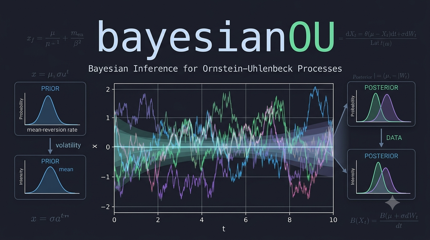
  • bayesianOU: Exploring Market Price Gravitation via Ornstein-Uhlenbeck Process

    bayesianOU: Exploring Market Price Gravitation via Ornstein-Uhlenbeck Process

    You can also find this library at CRAN and download it directly from R and RStudio.

    When Market Prices Gravitate: A Bayesian Look at an Old Question in Economics

    An old question, asked again — properly

    There is a question in economics that is older than most of the academic disciplines that border it. Do market prices — the noisy, day-to-day, here-and-now prices at which goods actually change hands — tend to settle toward some underlying center of gravity? And if they do, how fast, how violently, and through what mechanism?

    Classical political economy, from Smith and Ricardo through Marx, thought they do. The idea was that behind the churning surface of market prices there sit “prices of production”: long-run, cost-anchored prices toward which actual prices are pulled, the way a spring pulls a weight back toward its rest position. In the Marxian version, there is one more layer underneath: those prices of production themselves are supposed to gravitate around “values,” the labour embodied in commodities. Whether any of this is true is an empirical question, and for a long time the empirical tools to answer it were not really up to the job.

    A small R package called bayesianOU, written by José Mauricio Gómez Julián and hosted on GitHub, takes a serious swing at that question. It is not the first attempt to test price gravitation statistically, but it is one of the most technically careful I have seen, and it is built in a way that is instructive far beyond the Marxian debate that motivates it. What follows is a walkthrough of what the package does, why it is interesting, and — just as importantly — where it honestly admits its own limits.

    The tool that makes it possible: the Ornstein-Uhlenbeck process

    Strip the economics away for a moment and the statistical core of the package is a workhorse object from physics: the Ornstein-Uhlenbeck (OU) process. Imagine a particle moving in a fluid, attached to a spring. Brownian motion jiggles it randomly; the spring pulls it back toward a fixed point. The further it drifts away, the harder the pull. The result is a wiggly series that never settles but always tends to settle — a mean-reverting random walk.

    The OU process is exactly the mathematical object you want when you suspect a variable is noisy but anchored. It has a “speed of reversion” (how hard the spring pulls) and an “equilibrium level” (where the spring’s rest point is). Estimate those, and you can say something quantitative about gravitation: not just “yes, prices come back,” but “they come back with a half-life of about nine years.”

    That number — the half-life — is the prize. It is the difference between “market prices eventually settle” (which could mean anything) and “market prices settle on a timescale comparable to a business cycle” (which is a falsifiable, interpretable claim).

    What the package actually builds

    The package fits, by Bayesian inference, a family of models built on the OU process but considerably richer than the textbook version. There are two first-class models, sharing one inference engine.

    The single-level model

    The first model asks: do market prices revert toward an equilibrium that is a function of the prices of production, and what does that reversion look like once we let it be nonlinear, volatile, heavy-tailed, and structurally heterogeneous across sectors?

    Each of those adjectives is doing real work, and each corresponds to a feature that simpler approaches handle poorly or not at all:

    • Nonlinear drift. A plain OU process pulls back with a force proportional to the deviation. The package allows a cubic correction, so the restoring force can strengthen super-linearly when prices are far from equilibrium. This matters: real markets may behave gently near the center and violently at the extremes, and a linear model cannot represent that.
    • Stochastic volatility. Financial data, and economic data generally, go through quiet stretches and turbulent ones. The package does not assume a single noise level; it lets the volatility itself wander over time, following its own mean-reverting process on the log-variance. This is the same idea that powers modern stochastic-volatility models in finance, and it is essential for not fooling yourself about the precision of your estimates.
    • Heavy tails. Economic shocks are not Gaussian. Crashes, booms, and policy shocks produce outliers that a normal distribution would call essentially impossible. The package uses Student-t innovations and estimates the degrees of freedom from the data, so the model can discover for itself just how fat-tailed the world is.
    • Hierarchical structure across sectors. An economy has dozens of sectors, and each one presumably has its own reversion speed, its own equilibrium, its own noise. Estimating each sector in isolation throws away the information that they are all part of the same economy. Estimating them all with one set of parameters pretends they are identical. The package takes the middle path — hierarchical, or “partial pooling,” priors — where each sector’s parameters are drawn from a shared distribution whose properties the model also estimates. Sectors borrow strength from one another without being forced into lockstep.
    • A time-varying coupling. This is the most economically loaded feature. The strength with which market prices track prices of production is allowed to depend on the aggregate profit rate (what the package calls TMG). When the general rate of profit is high, the pull of production prices on market prices may be one thing; when it is low, another. Whether that modulation exists, and in which direction, is a hypothesis the model can test rather than assume.

    All of this is estimated jointly, with full Bayesian uncertainty, using Stan’s Hamiltonian Monte Carlo sampler. You do not get a point estimate of the reversion speed; you get a posterior distribution, and from it a credible interval and a probability statement like “there is a 95% chance the half-life is between six and eighteen years.”

    The nested cascade

    The second model is the more ambitious one, and it is where the package earns its “nested” branding. Instead of market prices reverting to a fixed equilibrium, they revert to a latent production price — a hidden, unobserved series that itself evolves over time according to its own OU process, driven by the general profit rate. And, if you turn on the third level, that latent production price in turn gravitates around an observed “value” index built directly from labour-content accounting.

    So the full structure is a cascade: market price → latent production price → value. Each arrow is an OU reversion, each with its own speed, and the speeds are constrained so that the outer (market) layer reverts faster than the inner (production) layer — an economically natural separation of timescales, enforced softly so the data can push back.

    The reason this matters is that it converts a slogan — “prices of production gravitate around values” — into a literal statistical hierarchy that can be fit to data and compared against alternatives. The headline empirical result, from a fit to 37 US sectors over 1960–2020, is a value-coupling coefficient essentially equal to one, with the posterior probability of it being positive effectively equal to one. In plain terms: in standardized units, prices of production track labour values almost one-for-one. That is a found result, not an assumed one — the prior on the coupling was centred at zero, deliberately neutral.

    The inference engine, and why it is not a footnote

    It would be easy to glance at the model description, nod, and move on. But how these quantities are estimated is half of what makes the package serious, and it is worth a paragraph for readers who do not think about MCMC every day.

    Bayesian inference works by exploring the space of all parameter values consistent with both the data and the prior, and characterizing that space as a probability distribution. For models this complex — with latent volatility paths, hierarchical structure, and hundreds of parameters — you cannot do that with pencil and paper. You use a Markov chain Monte Carlo sampler, specifically Hamiltonian Monte Carlo, which borrows an idea from physics: give the parameter space a “potential energy” (the log-posterior) and a “kinetic energy” (a randomly chosen momentum), and let the system glide around the posterior like a ball rolling over a landscape.

    Stan’s NUTS sampler automates this about as well as it can be automated, and the package uses it with within-chain parallelism (via Stan’s reduce_sum) to handle the fact that the likelihood must be summed over many timepoints and sectors. The diagnostics — R-hat for chain agreement, effective sample size, divergence counts — are surfaced through a validate_ou_fit function, and the package is explicit that you should look at them before believing anything.

    Model comparison is done with PSIS-LOO, a clever technique that approximates leave-one-out cross-validation without refitting the model dozens of times, by reweighting the posterior draws using importance sampling. It is the modern standard, and the package is appropriately cautious about it: because the model has a latent volatility state at every observation, plain LOO is known to be optimistic, and the documentation says so plainly.

    The honesty that makes it credible

    Here is where the package surprised me, and here is why I think it deserves a wider audience than the Marxian-economics niche it lives in.

    A naïve reading of the results would be triumphant: the value coupling is one-to-one, the reversion exists, the half-life is about nine years. But the package’s own validation section does something rare. It runs the model against legitimate rivals on genuinely held-out data — a full decade, 2011 to 2020 — and reports, without spin, that a random walk beats the OU model at forecasting, that a no-gravitation restriction ties or beats it, and that the value term adds no detectable predictive density.

    That sounds like a refutation. The package argues, carefully, that it is nothing of the sort — and the argument is the most intellectually interesting thing here.

    The key move is to distinguish two different questions. One is structural: does a reversion mechanism exist, and how fast is it? The other is predictive: can you forecast next year’s price better than a naïve benchmark? These are related but not identical, and for a slow process they come apart in a specific, predictable way.

    If gravitation is real but slow — a half-life of nine years on a dataset whose test window is a decade — then over the forecast horizon the process looks, to first order, like a random walk. The reversion is there, but it is too weak to show up in a one-step or few-step prediction. The random walk, which assumes no reversion, will forecast almost as well, because over short horizons a barely-reverting process and a non-reverting one are nearly indistinguishable. So the random walk winning the forecasting horse race is not evidence against gravitation; it is evidence consistent with gravitation being slow.

    This is not special pleading. It is a logical point about what different functionals of a model can and cannot tell you. The structural parameters — estimated from the joint likelihood over the whole panel, borrowing strength across 37 sectors and 61 years — use far more information than any single-series forecast. They can pin down a central tendency that a univariate test cannot. And the package shows, through simulation-based calibration and adversarial negative controls, that the estimation pipeline does not manufacture gravitation when none is present: feed it a true random walk and it reports a half-life of about fifty years; feed it a null value-coupling and the posterior honestly covers zero.

    The low-kappa trap, and why it matters to everyone

    The package names a difficulty it calls the low-kappa trap, and it is worth understanding because it is a trap that catches far more than Marxian price theory.

    Kappa is the reversion speed. As kappa shrinks toward zero, the OU process approaches a pure random walk. The trouble is that there is no bright line separating “slow mean reversion” from “no mean reversion.” It is a continuum, and three distinct problems stack up exactly there:

    • Algebraically, reversion speed and discrete-time persistence are two sides of the same coin; kappa going to zero is the same as the autocorrelation going to one. There is no internal frontier.
    • Statistically, the power of a unit-root test — the standard tool for asking “is this a random walk?” — collapses exactly as the truth approaches the random walk boundary. With a finite sample and a half-life comparable to the sample length, the test simply cannot tell. This is a well-known result in econometrics, and it is why decades of “is the real exchange rate stationary?” papers argued past one another.
    • Numerically, if the reversion speed is parameterized to be strictly positive (as it must be, for the sampler to behave), then “the probability that kappa is greater than zero” is trivially one — it tells you nothing. The informative quantity is the half-life, and the probability that the half-life exceeds some sensible horizon.

    The package’s response to the trap is instructive. It does not pretend the trap is not there. It states all three layers explicitly, reports the slow tail honestly (one sector has a non-trivial posterior probability of a half-life beyond forty years), and argues that the joint hierarchical posterior — which pools information across the whole panel — is a more powerful discriminator than any univariate test. That is a defensible position, and it is stated with the caveat attached rather than buried in a footnote.

    This is the broader lesson. Anyone working with time series that might be slowly mean-reverting — interest rates, real exchange rates, commodity prices, climate variables, pollutant concentrations — runs into exactly this trap. The package’s framing of it, in three layers, is one of the clearest expositions I have read, and it would travel well into any of those domains.

    What I appreciate, and what I would watch for

    A few things stand out as genuinely good practice, and they are worth naming because they are rarer than they should be.

    The separation of economic and sampler convergence. The package is scrupulous about not confusing two senses of “convergence.” Economic convergence — does the price revert? — is a statement about kappa and the half-life. Sampler convergence — did the MCMC chains agree? — is a statement about R-hat and divergences. These share a word and nothing else, and conflating them is a classic source of muddled reasoning. The documentation keeps them lexically distinct throughout.

    Neutral priors on the load-bearing hypotheses. The prior on the profit-rate modulation is centred at zero. The prior on the value coupling is centred at zero. The package does not bake the answer into the question. When the posterior then moves clearly away from zero, that means something.

    Out-of-sample integrity by construction. A subtle and common error in time-series work is “leakage”: accidentally letting future information contaminate the training procedure, so that out-of-sample results are secretly in-sample. The package offers a fit_window switch that keeps the two designs genuinely separate, and it computes the common-factor loadings from the training window only. This is the kind of plumbing detail that separates trustworthy work from work that just looks trustworthy.

    The negative results are reported. Many packages, and most blog posts about them, would quietly omit the fact that a random walk out-forecasts the model. This one leads with it and then reasons about it. That is how a field accumulates reliable knowledge rather than just encouraging headlines.

    What should a careful reader watch for? The half-life estimate of about nine years is, by the package’s own account, probably conservatively slow — a controlled study of the disaggregation step suggests the true figure may be closer to seven or eight. The cubic nonlinearity is a minor refinement on this data (its coefficient sits near its prior). The Student-t degrees of freedom and the stochastic-volatility scale are weakly identified when both are present, a known tension the documentation flags but does not resolve. And the headline value-coupling result, while striking, is measured on standardized levels that share a cost-price component by construction; the package defends this with a “wedge” argument — subtracting the shared component and testing the residual — but a sceptical reader should follow that argument itself rather than take it on trust.

    None of these caveats undermine the project. They are the project. A statistical framework that cannot articulate its own soft spots is not a framework you should believe.

    Why it is worth your time

    You do not need to be a Marxian economist, or any kind of economist, to get something out of this package. If you work with time series that exhibit slow, noisy reversion toward a moving target — and a great deal of the physical and social world does — the modelling ideas here are directly portable: the nonlinear OU drift, the stochastic volatility, the hierarchical pooling across groups, the careful separation of structural estimation from forecasting, and the three-layer diagnosis of the low-reversion trap.

    And if you are interested in the classical question of whether prices gravitate toward values, this is about as good a statistical treatment as you will find: modern machinery, honest reporting, and a willingness to let the data argue back against the theory that motivated the exercise in the first place.

    The repository, the full mathematical specification, the validation blocks, and a frank discussion of every methodological decision live at github.com/IsadoreNabi/bayesianOU, with the wiki carrying the complete technical detail. Read the methodology notes before you quote a number; that is what they are there for.