You can also find this library at CRAN and download it directly from R and RStudio.

LISTEN TO THIS POST AS A PODCAST:

When Market Prices Gravitate: A Bayesian Look at an Old Question in Economics

An old question, asked again — properly

There is a question in economics that is older than most of the academic disciplines that border it. Do market prices — the noisy, day-to-day, here-and-now prices at which goods actually change hands — tend to settle toward some underlying center of gravity? And if they do, how fast, how violently, and through what mechanism?

Classical political economy, from Smith and Ricardo through Marx, thought they do. The idea was that behind the churning surface of market prices there sit “prices of production”: long-run, cost-anchored prices toward which actual prices are pulled, the way a spring pulls a weight back toward its rest position. In the Marxian version, there is one more layer underneath: those prices of production themselves are supposed to gravitate around “values,” the labour embodied in commodities. Whether any of this is true is an empirical question, and for a long time the empirical tools to answer it were not really up to the job.

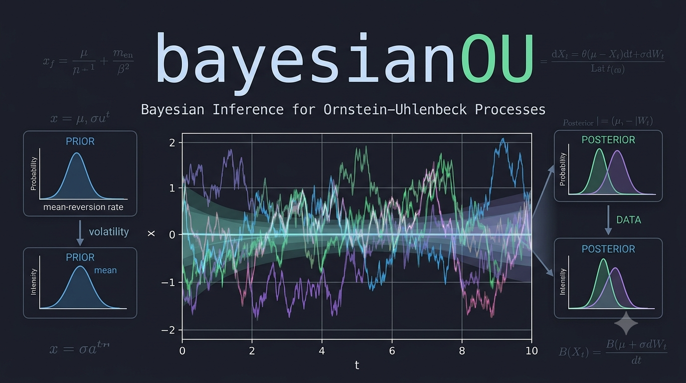
A small R package called bayesianOU, written by José Mauricio Gómez Julián and hosted on GitHub, takes a serious swing at that question. It is not the first attempt to test price gravitation statistically, but it is one of the most technically careful I have seen, and it is built in a way that is instructive far beyond the Marxian debate that motivates it. What follows is a walkthrough of what the package does, why it is interesting, and — just as importantly — where it honestly admits its own limits.

The tool that makes it possible: the Ornstein-Uhlenbeck process

Strip the economics away for a moment and the statistical core of the package is a workhorse object from physics: the Ornstein-Uhlenbeck (OU) process. Imagine a particle moving in a fluid, attached to a spring. Brownian motion jiggles it randomly; the spring pulls it back toward a fixed point. The further it drifts away, the harder the pull. The result is a wiggly series that never settles but always tends to settle — a mean-reverting random walk.

The OU process is exactly the mathematical object you want when you suspect a variable is noisy but anchored. It has a “speed of reversion” (how hard the spring pulls) and an “equilibrium level” (where the spring’s rest point is). Estimate those, and you can say something quantitative about gravitation: not just “yes, prices come back,” but “they come back with a half-life of about nine years.”

That number — the half-life — is the prize. It is the difference between “market prices eventually settle” (which could mean anything) and “market prices settle on a timescale comparable to a business cycle” (which is a falsifiable, interpretable claim).

What the package actually builds

The package fits, by Bayesian inference, a family of models built on the OU process but considerably richer than the textbook version. There are two first-class models, sharing one inference engine.

The single-level model

The first model asks: do market prices revert toward an equilibrium that is a function of the prices of production, and what does that reversion look like once we let it be nonlinear, volatile, heavy-tailed, and structurally heterogeneous across sectors?

Each of those adjectives is doing real work, and each corresponds to a feature that simpler approaches handle poorly or not at all:

• Nonlinear drift. A plain OU process pulls back with a force proportional to the deviation. The package allows a cubic correction, so the restoring force can strengthen super-linearly when prices are far from equilibrium. This matters: real markets may behave gently near the center and violently at the extremes, and a linear model cannot represent that.
• Stochastic volatility. Financial data, and economic data generally, go through quiet stretches and turbulent ones. The package does not assume a single noise level; it lets the volatility itself wander over time, following its own mean-reverting process on the log-variance. This is the same idea that powers modern stochastic-volatility models in finance, and it is essential for not fooling yourself about the precision of your estimates.
• Heavy tails. Economic shocks are not Gaussian. Crashes, booms, and policy shocks produce outliers that a normal distribution would call essentially impossible. The package uses Student-t innovations and estimates the degrees of freedom from the data, so the model can discover for itself just how fat-tailed the world is.
• Hierarchical structure across sectors. An economy has dozens of sectors, and each one presumably has its own reversion speed, its own equilibrium, its own noise. Estimating each sector in isolation throws away the information that they are all part of the same economy. Estimating them all with one set of parameters pretends they are identical. The package takes the middle path — hierarchical, or “partial pooling,” priors — where each sector’s parameters are drawn from a shared distribution whose properties the model also estimates. Sectors borrow strength from one another without being forced into lockstep.
• A time-varying coupling. This is the most economically loaded feature. The strength with which market prices track prices of production is allowed to depend on the aggregate profit rate (what the package calls TMG). When the general rate of profit is high, the pull of production prices on market prices may be one thing; when it is low, another. Whether that modulation exists, and in which direction, is a hypothesis the model can test rather than assume.

All of this is estimated jointly, with full Bayesian uncertainty, using Stan’s Hamiltonian Monte Carlo sampler. You do not get a point estimate of the reversion speed; you get a posterior distribution, and from it a credible interval and a probability statement like “there is a 95% chance the half-life is between six and eighteen years.”

The nested cascade

The second model is the more ambitious one, and it is where the package earns its “nested” branding. Instead of market prices reverting to a fixed equilibrium, they revert to a latent production price — a hidden, unobserved series that itself evolves over time according to its own OU process, driven by the general profit rate. And, if you turn on the third level, that latent production price in turn gravitates around an observed “value” index built directly from labour-content accounting.

So the full structure is a cascade: market price → latent production price → value. Each arrow is an OU reversion, each with its own speed, and the speeds are constrained so that the outer (market) layer reverts faster than the inner (production) layer — an economically natural separation of timescales, enforced softly so the data can push back.

The reason this matters is that it converts a slogan — “prices of production gravitate around values” — into a literal statistical hierarchy that can be fit to data and compared against alternatives. The headline empirical result, from a fit to 37 US sectors over 1960–2020, is a value-coupling coefficient essentially equal to one, with the posterior probability of it being positive effectively equal to one. In plain terms: in standardized units, prices of production track labour values almost one-for-one. That is a found result, not an assumed one — the prior on the coupling was centred at zero, deliberately neutral.

The inference engine, and why it is not a footnote

It would be easy to glance at the model description, nod, and move on. But how these quantities are estimated is half of what makes the package serious, and it is worth a paragraph for readers who do not think about MCMC every day.

Bayesian inference works by exploring the space of all parameter values consistent with both the data and the prior, and characterizing that space as a probability distribution. For models this complex — with latent volatility paths, hierarchical structure, and hundreds of parameters — you cannot do that with pencil and paper. You use a Markov chain Monte Carlo sampler, specifically Hamiltonian Monte Carlo, which borrows an idea from physics: give the parameter space a “potential energy” (the log-posterior) and a “kinetic energy” (a randomly chosen momentum), and let the system glide around the posterior like a ball rolling over a landscape.

Stan’s NUTS sampler automates this about as well as it can be automated, and the package uses it with within-chain parallelism (via Stan’s reduce_sum) to handle the fact that the likelihood must be summed over many timepoints and sectors. The diagnostics — R-hat for chain agreement, effective sample size, divergence counts — are surfaced through a validate_ou_fit function, and the package is explicit that you should look at them before believing anything.

Model comparison is done with PSIS-LOO, a clever technique that approximates leave-one-out cross-validation without refitting the model dozens of times, by reweighting the posterior draws using importance sampling. It is the modern standard, and the package is appropriately cautious about it: because the model has a latent volatility state at every observation, plain LOO is known to be optimistic, and the documentation says so plainly.

The honesty that makes it credible

Here is where the package surprised me, and here is why I think it deserves a wider audience than the Marxian-economics niche it lives in.

A naïve reading of the results would be triumphant: the value coupling is one-to-one, the reversion exists, the half-life is about nine years. But the package’s own validation section does something rare. It runs the model against legitimate rivals on genuinely held-out data — a full decade, 2011 to 2020 — and reports, without spin, that a random walk beats the OU model at forecasting, that a no-gravitation restriction ties or beats it, and that the value term adds no detectable predictive density.

That sounds like a refutation. The package argues, carefully, that it is nothing of the sort — and the argument is the most intellectually interesting thing here.

The key move is to distinguish two different questions. One is structural: does a reversion mechanism exist, and how fast is it? The other is predictive: can you forecast next year’s price better than a naïve benchmark? These are related but not identical, and for a slow process they come apart in a specific, predictable way.

If gravitation is real but slow — a half-life of nine years on a dataset whose test window is a decade — then over the forecast horizon the process looks, to first order, like a random walk. The reversion is there, but it is too weak to show up in a one-step or few-step prediction. The random walk, which assumes no reversion, will forecast almost as well, because over short horizons a barely-reverting process and a non-reverting one are nearly indistinguishable. So the random walk winning the forecasting horse race is not evidence against gravitation; it is evidence consistent with gravitation being slow.

This is not special pleading. It is a logical point about what different functionals of a model can and cannot tell you. The structural parameters — estimated from the joint likelihood over the whole panel, borrowing strength across 37 sectors and 61 years — use far more information than any single-series forecast. They can pin down a central tendency that a univariate test cannot. And the package shows, through simulation-based calibration and adversarial negative controls, that the estimation pipeline does not manufacture gravitation when none is present: feed it a true random walk and it reports a half-life of about fifty years; feed it a null value-coupling and the posterior honestly covers zero.

The low-kappa trap, and why it matters to everyone

The package names a difficulty it calls the low-kappa trap, and it is worth understanding because it is a trap that catches far more than Marxian price theory.

Kappa is the reversion speed. As kappa shrinks toward zero, the OU process approaches a pure random walk. The trouble is that there is no bright line separating “slow mean reversion” from “no mean reversion.” It is a continuum, and three distinct problems stack up exactly there:

• Algebraically, reversion speed and discrete-time persistence are two sides of the same coin; kappa going to zero is the same as the autocorrelation going to one. There is no internal frontier.
• Statistically, the power of a unit-root test — the standard tool for asking “is this a random walk?” — collapses exactly as the truth approaches the random walk boundary. With a finite sample and a half-life comparable to the sample length, the test simply cannot tell. This is a well-known result in econometrics, and it is why decades of “is the real exchange rate stationary?” papers argued past one another.
• Numerically, if the reversion speed is parameterized to be strictly positive (as it must be, for the sampler to behave), then “the probability that kappa is greater than zero” is trivially one — it tells you nothing. The informative quantity is the half-life, and the probability that the half-life exceeds some sensible horizon.

The package’s response to the trap is instructive. It does not pretend the trap is not there. It states all three layers explicitly, reports the slow tail honestly (one sector has a non-trivial posterior probability of a half-life beyond forty years), and argues that the joint hierarchical posterior — which pools information across the whole panel — is a more powerful discriminator than any univariate test. That is a defensible position, and it is stated with the caveat attached rather than buried in a footnote.

This is the broader lesson. Anyone working with time series that might be slowly mean-reverting — interest rates, real exchange rates, commodity prices, climate variables, pollutant concentrations — runs into exactly this trap. The package’s framing of it, in three layers, is one of the clearest expositions I have read, and it would travel well into any of those domains.

What I appreciate, and what I would watch for

A few things stand out as genuinely good practice, and they are worth naming because they are rarer than they should be.

The separation of economic and sampler convergence. The package is scrupulous about not confusing two senses of “convergence.” Economic convergence — does the price revert? — is a statement about kappa and the half-life. Sampler convergence — did the MCMC chains agree? — is a statement about R-hat and divergences. These share a word and nothing else, and conflating them is a classic source of muddled reasoning. The documentation keeps them lexically distinct throughout.

Neutral priors on the load-bearing hypotheses. The prior on the profit-rate modulation is centred at zero. The prior on the value coupling is centred at zero. The package does not bake the answer into the question. When the posterior then moves clearly away from zero, that means something.

Out-of-sample integrity by construction. A subtle and common error in time-series work is “leakage”: accidentally letting future information contaminate the training procedure, so that out-of-sample results are secretly in-sample. The package offers a fit_window switch that keeps the two designs genuinely separate, and it computes the common-factor loadings from the training window only. This is the kind of plumbing detail that separates trustworthy work from work that just looks trustworthy.

The negative results are reported. Many packages, and most blog posts about them, would quietly omit the fact that a random walk out-forecasts the model. This one leads with it and then reasons about it. That is how a field accumulates reliable knowledge rather than just encouraging headlines.

What should a careful reader watch for? The half-life estimate of about nine years is, by the package’s own account, probably conservatively slow — a controlled study of the disaggregation step suggests the true figure may be closer to seven or eight. The cubic nonlinearity is a minor refinement on this data (its coefficient sits near its prior). The Student-t degrees of freedom and the stochastic-volatility scale are weakly identified when both are present, a known tension the documentation flags but does not resolve. And the headline value-coupling result, while striking, is measured on standardized levels that share a cost-price component by construction; the package defends this with a “wedge” argument — subtracting the shared component and testing the residual — but a sceptical reader should follow that argument itself rather than take it on trust.

None of these caveats undermine the project. They are the project. A statistical framework that cannot articulate its own soft spots is not a framework you should believe.

Why it is worth your time

You do not need to be a Marxian economist, or any kind of economist, to get something out of this package. If you work with time series that exhibit slow, noisy reversion toward a moving target — and a great deal of the physical and social world does — the modelling ideas here are directly portable: the nonlinear OU drift, the stochastic volatility, the hierarchical pooling across groups, the careful separation of structural estimation from forecasting, and the three-layer diagnosis of the low-reversion trap.

And if you are interested in the classical question of whether prices gravitate toward values, this is about as good a statistical treatment as you will find: modern machinery, honest reporting, and a willingness to let the data argue back against the theory that motivated the exercise in the first place.

The repository, the full mathematical specification, the validation blocks, and a frank discussion of every methodological decision live at github.com/IsadoreNabi/bayesianOU, with the wiki carrying the complete technical detail. Read the methodology notes before you quote a number; that is what they are there for.