“Is that to say we are against Free Trade? No, we are for Free Trade, because by Free Trade all economical laws, with their most astounding contradictions, will act upon a larger scale, upon the territory of the whole earth; and because from the uniting of all these contradictions in a single group, where they will stand face to face, will result the struggle which will itself eventuate in the emancipation of the proletariat.”
Karl Heinrich Marx · Marx-Engels Collected Works, Vol. VI, p. 290
You can also find this library at CRAN and download it directly from R and RStudio.
Also, we recommend viewing the mind map summary at the end of the article to better understand the relationship between the functions of the package.
LISTEN TO THIS POST AS A PODCAST:
ESCUCHA ESTA PUBLICACIÓN COMO PODCAST
R Library Review
Meet gdpar
General Dynamic Parameter Models via Reference Anchoring
In the fleeting calculus of a two-second decision—overtaking a car on a narrow road—the human brain performs a remarkable statistical trick. It does not build a model of the approaching driver from scratch. Instead, it retrieves a baseline: the average driver, representing typical reaction times and modal aggression. In a split second, it reads the specific signals of the actual driver—relative speed, vehicle type, micro-movements—and estimates how this specific driver deviates from the baseline. The decision to overtake emerges from that synthesis.
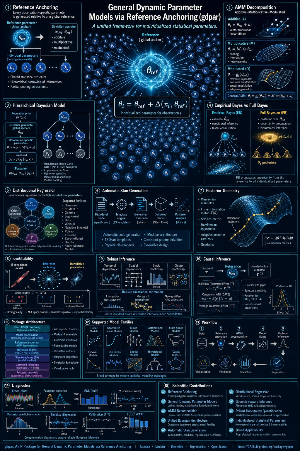
This cognitive recipe—population reference + individual deviation—is the philosophical bedrock of the R package gdpar (General Dynamic Parameter models via Reference Anchoring) by José Mauricio Gómez Julián. The package takes this intuition, formalizes it as a rigorous statistical decomposition, proves the conditions under which it is mathematically identifiable, ships a Stan-based Bayesian engine to estimate it, and layers on causal inference, geometry-adaptive sampling, and dependence-robust inference.
❦
The Anatomy of Deviation
Every layer of gdpar is an elaboration of a single, elegant equation. For each observation $i$ with covariates $x_i$:
Read it as: the parameter of individual $i$ equals a population reference, plus a deviation that is itself a function of the individual’s covariates and of the reference itself.
That final clause is where the architecture pivots from classical statistics. The deviation $\Delta$ does not merely depend on who you are (your covariates $x_i$); it depends on what the reference is. If you transplant the model to a new population, the deviation function behaves differently because $\theta_{\text{ref}}$ is one of its arguments. This structural dependence is the defining feature of “reference anchoring.” It distinguishes gdpar from random-effects or varying-coefficient models, where the deviation is structurally separate from the reference.
So, what is the shape of $\Delta$? The package singles out a specific functional form called the Additive–Multiplicative–Modulated (AMM) decomposition:
Three mechanisms, cleanly separated and independently interpretable:
$a(x)$ — A pure additive shift. Think of this as a traditional fixed-effect driven by covariates.
$b(x)\odot\theta_{\text{ref}}$ — A covariate-dependent scaling of the reference (using the Hadamard/elementwise product). This is where “the deviation depends on the reference” enters multiplicatively.
$W(\theta_{\text{ref}})\,x$ — Covariates are mixed through a matrix $W$ that is, itself, tuned by the reference. This is the explicit, structural reference-dependent channel.
Standard models drop out as special cases. Set $\Delta \equiv 0$ and you have fixed-effects regression. Set $W \equiv 0$ and you have a hierarchical model with multiplicative interaction. Set $b \equiv 0$ and you have a varying-coefficient model. The AMM is the smallest natural family that contains all three and elevates the reference to an active argument of the deviation.
❦
The Three Estimation Engines
gdpar defines three complementary engines for estimating $\Delta$. Crucially, only one is executable in the current release—a deliberate choice to promise a mathematical scope that exceeds the executable surface, and to say so honestly.
Path
Engine
Representation
Status
Path 1
Hierarchical Bayesian (Stan)
Parametric AMM
✅ Operational
Path 2
Varying-coefficient (splines)
Smooth $\beta(z)$
🚧 Conceptual
Path 3
Hypernetwork / Neural Net
Net generates $\theta_i$
🚧 Conceptual
Paths 2 and 3 are documented to “reference grade”—full asymptotic theory (contraction rates, Bernstein–von Mises) is developed in the Wiki—but they abort with gdpar_unsupported_feature_error if invoked. Path 1 places priors on every component ($\theta_{\text{ref}}, a, b, W$) and samples the joint posterior with HMC, yielding native, full-posterior uncertainty.
A Tale of Two Posteriors: EB vs. FB
Within Path 1, gdpar offers two inferential regimes. Full Bayes (FB) via gdpar() samples the joint posterior, remaining most faithful to the cognitive analogy. Empirical Bayes (EB) via gdpar_eb() estimates the hyperparameters by maximizing a marginal likelihood via a Laplace approximation, then samples the remaining parameters conditionally.
The EB vs FB Comparator
Rather than forcing a choice, gdpar treats them as parallel routes. It ships a dedicated comparator, gdpar_compare_eb_fb(), which quantifies agreement on $\theta_{\text{ref}}$ and the reduced parameter vector $\xi$. The Wiki develops the theory to first-class depth: EB and FB lower-level posteriors agree asymptotically (Theorem 7A), while EB intervals under-cover by $O(n^{-1})$ (Proposition 7B). If you have ever wondered if EB is “good enough” for your data, gdpar lets you answer that empirically.
Distributional Regression: Every Parameter is a Slot
gdpar is not constrained to modeling the mean. A probability distribution has multiple parameters—location, scale, shape, tail index, zero-inflation probability—and each one can carry its own AMM decomposition. The package indexes these by $k = 1, \dots, K$:
$$ \theta_i^{(k)} = \theta_{\text{ref}}^{(k)} + \Delta^{(k)}(x_i, \theta_{\text{ref}}^{(k)}), \qquad k = 1, \dots, K $$
The built-in roster covers Gaussian, Poisson, negative binomial, Bernoulli, Beta, Gamma, Student-$t$, Tweedie, ZIP, ZINB, and hurdle families. Zero-inflated and hurdle models receive an especially elegant treatment: both the zero-inflation probability $\pi_i$ and the count parameter $\theta_i$ are anchored to their respective references—a dual deviation design.
❦
The Causal Bridge
Because the AMM form produces individual parameters, individual treatment effects emerge naturally. gdpar_causal_bridge() implements a T-learner: fit the anchored model separately under treatment and control, then read the conditional average treatment effect (CATE) at $x_i$ as the difference of the anchored individual predictions:
A second layer, gdpar_compare_meta_learners(), benchmarks the AMM-based learner against external meta-learners via pluggable adapters: grf::causal_forest on the R side and EconML’s CausalForestDML on the Python side (via reticulate). The framework’s causal claims are benchmarked, not asserted.
Mechanics & Clockwork
Several engineering decisions elevate gdpar from a theoretical exercise to a serious computational environment:
Stan Code Generator: Composes programs from canonical pieces—AMM blocks for $p=1$ and $p \geq 1$, EB marginal/conditional blocks, distributional-$K$ blocks—selected by the resolved $(K, p, \text{family}, W, \text{parametrization}, \text{group})$. The $W$ basis supports B-splines with Stan-side Cox–de Boor evaluation, ensuring differentiability inside HMC.
Identifiability Pre-flight: Before any sampling, gdpar_check_identifiability() runs a Gram-matrix check (Proposition 1C), a per-coordinate cross-component check (C4-bis) for $p > 1$, and a per-group anti-aliasing check (C7). If your design is non-identifiable, you find out before the sampler burns your CPU, accompanied by a structured gdpar_identifiability_error naming the dependent directions.
Data-Driven Reparametrization: Treats the parametrization of $b(x) \odot \theta_{\text{ref}}$ as a pre-fit decision. A short pilot computes an information ratio, dispatching to CP, NCP, or—gdpar‘s root-cause resolution—a linear reparametrization that samples the product $\theta_{\text{ref}} \cdot b$ directly, sidestepping bilinear funnels altogether.
Opt-in Power Tools
Two advanced capabilities are switched off by default, documented as thoroughly as the core path.
1. Geometry-Adaptive Sampling
Hierarchical AMM posteriors can be geometrically hostile—funnels, near-determinism, heavy tails. The opt-in geometry engine climbs a ladder of Riemannian metrics: Euclidean → Fisher/SoftAbs → sub-Riemannian → relativistic/Finsler. A certifying orchestrator diagnoses the pathology, selects a metric, tunes the integrator, and emits a certificate. If full sampling is certified infeasible, a Laplace fallback provides a plug-in posterior with ELPD on par with mgcv-REML or INLA-Laplace.
2. Dependence-Robust Inference
gdpar does not model temporal or spatial dependence in its point structure; instead, it makes the inference robust to dependence (a working-independence + sandwich-variance stance in the spirit of Liang & Zeger, 1986). You receive diagnostics (Durbin–Watson, Ljung–Box, Moran’s $I$) and robust SEs via block bootstrap—moving or circular blocks in time (with the Politis–White flat-top automatic block length), tiled randomized-origin blocks in space. Point estimates remain pristine; only the uncertainty is made honest.
⚠️ Honest Limitations
The Wiki is admirably forthright about scope. Only Path 1 is executable in 0.1.0. Dependence is not modelled—only the inference is made robust. The package’s mathematical scope exceeds its executable surface by design. Read the “Implementation status” notes carefully before relying on a feature.
❦
TL;DR
gdpar takes one of the most natural ideas in human prediction—predict an individual as a deviation from a population reference, where the deviation itself depends on the reference—and transforms it into a fully specified, identifiability-checked, Stan-powered Bayesian regression framework. It is theoretically rigorous, computationally serious, and unusually honest about what it does and does not yet do. If your work involves individual heterogeneity, distributional regression, or causal effect estimation with principled uncertainty, gdpar demands a careful look.
You can also find this libraryat CRAN and download it directly from R and RStudio.
LISTEN TO THIS POST AS A PODCAST:
You have a national Consumer Price Index. It is a single number per year. What you actually want is the price index for each sector of the economy — manufacturing, services, agriculture, construction — because those individual paths are what your model, your policy analysis, or your investment thesis really needs. You know how the sectors combine into the whole: the weights are public, or at least knowable. What you do not know is the sectoral numbers themselves. You only ever see their weighted sum.
This is the disaggregation problem. It sounds like bookkeeping. It is actually a quietly profound statistical question, and the R package BayesianDisaggregation — built by José Mauricio Gómez Julián — tackles it with a degree of intellectual honesty that is rare in software. This post is a deep, plain-language tour of what the package does, why it works the way it does, and what it teaches about building statistical tools that tell the truth.
If you want to follow along with the code, the project’s wiki has installation instructions, function references, and worked examples. This post deliberately stays code-free so the ideas come through.
The problem, precisely
Let’s make it concrete. You observe an aggregate index — call it the CPI — over T years. You also have a matrix of weights W: for each year and each of K sectors, W tells you that sector’s share of the total. The weights sum to one within each year. The aggregate is, up to measurement noise, the weighted sum of the latent sectoral indices:
CPI at year t ≈ the weighted sum of the K sectoral indices, using that year’s weights.
The goal: recover the K sectoral indices — call them φ — from the single aggregate series and the known weights.
Here is the catch, and it is the entire heart of the matter. At every single year, the aggregate pins down one linear combination of the K sectors. The remaining K−1 directions are completely unconstrained by the data. With four sectors, you have one equation and four unknowns per year. The system is, in a precise mathematical sense, under-determined.
This is not a numerical annoyance you can engineer away. It is structural. Any method that hands you a single, sharp sectoral path from an aggregate alone is, whether it admits it or not, smuggling in assumptions to fill the gap — and most methods do not tell you how much of the answer is data and how much is assumption.
The question is not can you disaggregate. You always can. The question is: can you do it honestly, showing your work, and carrying the right amount of uncertainty forward?
The wrong way: a cautionary tale
The first version of the package — the 0.1.x line — advertised “MCMC-free Bayesian disaggregation.” The pitch was appealing: no slow Markov chain Monte Carlo sampling, just clean closed-form math. The implementation used a family of deterministic update rules — weighted, multiplicative, Dirichlet, adaptive — over the prior weight matrix.
It did not work. Not in the sense of crashing. In the much more dangerous sense of appearing to work while silently not doing the one thing it claimed to do.
The package’s own author, in a moment of radical honesty that is worth pausing on, audited the 0.1.x family and catalogued six foundational defects, labeled F1 through F6:
F1 — the aggregate never entered the computation. The “posterior” was derived entirely from the prior weight matrix. The actual observed CPI — the one piece of real evidence — was never used. The method was not conditioning on data; it was rearranging priors.
F2 — the Dirichlet concentration cancelled on renormalization. A parameter that was supposed to control how concentrated the sectoral estimates were simply vanished in the algebra when weights were normalized to sum to one.
F3 — the temporal pattern cancelled too. A component meant to encode smoothness over time also disappeared in the renormalization.
F4 — the “efficiency” term was a fixed constant. It looked like a data-dependent quality score; it was actually invariant.
F5 — there were no recovery tests. No one had ever generated synthetic data with a known truth and checked whether the method got it back.
F6 — a correlation helper cheated. It computed both Pearson and Spearman correlation and reported whichever was larger, a form of silent data-snooping.
The most damning of these is F1. A Bayesian method that does not condition on data is not a Bayesian method. It is a deterministic transformation dressed in Bayesian vocabulary. And the worst part is that it looked reasonable — it returned numbers, they moved in plausible directions, and nothing crashed.
The author’s response is, I think, the most important thing about this whole project. Rather than patching the defects one by one — adding the CPI here, fixing the concentration there — the author recognized that the foundational problem (not using the data) cannot be fixed within a deterministic re-weighting framework. The fix is not a patch. The fix is a fundamentally different model: one in which the aggregate enters as genuine evidence.
So the entire 0.1.x family was deleted. Every function — bayesian_disaggregate(), compute_L_from_P(), spread_likelihood(), the four update rules, the grid search, the save function, the cheating correlation helper — all of it, gone. In its place: two Bayesian engines that actually condition on the data. The package version jumped to 0.2.0, the DESCRIPTION was edited to remove any claim of novelty, and the documentation was rewritten to be explicit about what was removed and why.
This is what intellectual honesty in software looks like. It is not common. We should notice it when it happens.
The right idea: the aggregate as evidence
The conceptual move is simple to state and deep in consequence. Instead of treating the relationship between the aggregate and the sectors as a renormalization identity — a bit of algebra you apply after the fact — treat it as an observation density. The aggregate CPI is data. It is evidence about the latent sectors. The model should condition on it.
In the package’s canonical engine, this means: the latent sectoral indices φ evolve over time as a random walk with drift, and the observed CPI is generated from the weighted sum of the sectors with some observation noise. The aggregate is not a constraint imposed after estimation; it is the likelihood. The sectors come out the other side as a posterior distribution — not a single number, but a full cloud of plausible values with credible intervals.
This is the difference between solving an equation and updating beliefs in light of evidence. The first gives you a point. The second gives you a distribution. And as we will see, the distribution is the whole point.
Two engines, one trade-off
The package offers two ways to do the Bayesian inference, and the choice between them is a clean, well-explained trade-off between richness and exactness.
The state-space MCMC engine
This is the canonical, full-featured model. The sectoral indices live in log space, which guarantees they stay positive — a natural constraint for price indices that a model in raw levels could violate. Each sector’s log-index follows a random walk with its own drift and its own innovation scale (the amount of jitter per period).
Two layers of hierarchical structure make this more than K independent random walks:
Partial pooling on the drift. Each sector has its own drift, but the drifts are drawn from a common distribution. This means sectors share information about their average growth rate without being forced to be identical — the classic shrinkage trade-off.
Partial pooling on the innovation scale. Similarly, each sector’s volatility is drawn from a shared distribution. Sectors borrow strength in estimating how jittery they are.
The initial cross-section — the starting levels of the sectors at the first period — is anchored at the aggregate level with an estimable dispersion parameter. This is a subtle but important point. In the old, broken 0.1.x family, the “concentration” parameter was supposed to control how spread out the sectors were, but it cancelled in the algebra and had no effect. In the new model, the dispersion is a genuine parameter that the data and priors can actually estimate. It does not cancel. It does real work.
Finally, the observation: the CPI is modeled as coming from a Student-t distribution centered at the weighted sum of the sectors, with an estimable scale. The Student-t (rather than a Gaussian) makes the model robust to outliers in the aggregate — a heavy-tailed observation can be accommodated without wrecking the fit. If you prefer, you can switch to a plain Gaussian observation.
Because this model is not conjugate — the log transform, the Student-t, and the hierarchical structure break the neat algebra that would allow a closed-form solution — it is fit by Hamiltonian Monte Carlo via Stan (using either the cmdstanr or rstan backend). HMC is the gold standard for this kind of model: it handles the correlated, high-dimensional parameter space efficiently and comes with reliable diagnostics. The package runs four chains by default, checks the R-hat convergence statistic and the number of divergent transitions, and returns posterior draws of every sectoral index at every period.
The closed-form conjugate engine
The second engine is the linear-Gaussian counterpart. The sectoral indices evolve as a random walk in levels (not logs), and the aggregate is observed with Gaussian noise. This model is conjugate, which means its exact posterior can be computed in closed form — no MCMC, no sampling, no convergence diagnostics. The tool is the Kalman filter combined with the Rauch-Tung-Striebel smoother: the filter passes forward through time, updating beliefs about the sectors given each new CPI observation, and the smoother passes backward, refining those beliefs using future information.
If you want joint posterior draws — not just the smoothed means and variances, but actual correlated samples from the full posterior — the package uses the Durbin-Koopman simulation smoother, a elegant technique that produces draws with the correct cross-time and cross-sector covariance structure. These draws are not marginal approximations; they are genuine samples from the joint posterior.
This engine is the “correct realization of the original MCMC-free posterior idea.” The 0.1.x family wanted a closed-form Bayesian answer; the problem was not that closed-form is un-Bayesian (conjugacy is perfectly Bayesian), but that the old method did not use the data. This engine uses the data — the aggregate enters as the observation equation — and it does so in exact, closed form.
The trade-off is explicit and documented. The closed-form engine buys you speed and mathematical exactness. It costs you three things: positivity (levels can drift slightly negative, which logs prevent), robustness (Gaussian observations are sensitive to outliers, which the Student-t handles), and the cross-sector hierarchy (there is no partial pooling in the linear-Gaussian model). The MCMC engine buys you all three of those, at the cost of sampling.
Both engines return the same thing: an array of posterior draws of the sectoral indices, with dimensions [periods × sectors × draws], plus summary tables of medians and 95% credible bands.
The honesty at the center: weak identification
Here is where the package earns its deepest respect. It would be tempting, after building a real Bayesian model that conditions on the data, to declare victory and hand users sharp sectoral estimates. The package does not do this. Instead, it is explicit about a fact that most disaggregation methods gloss over: the sectoral split is only weakly identified.
Remember the under-determination: at each period, the aggregate pins down one linear combination of the K sectors. The remaining K−1 directions are governed by the prior — the cross-sectional dispersion and the temporal smoothness — not by the data. This means the posterior intervals for individual sectors are wide, and they are influenced by the prior. This is not a bug. It is not a limitation to be engineered away. It is the correct representation of what the data can and cannot tell you.
The package’s own recovery tests — which generate synthetic data from the model’s own data-generating process, where the true sectoral paths are known — confirm this directly. The aggregate is recovered essentially perfectly: the correlation between the fitted aggregate and the true aggregate is above 0.95, often essentially 1.0. The aggregate is strongly identified. But the sectoral coverage — the fraction of times the true sectoral path falls within the 95% credible band — is around 0.84, with the bands being deliberately wide. The test asserts that coverage exceeds 0.70, a conservative threshold, because the package refuses to claim sectoral precision that the data cannot deliver.
This is “rigour by layers”: assert tightly what is identified, assert conservatively what is not. It would be easy to tune the prior to produce narrower, more impressive-looking bands. The package deliberately does not.
Why the full posterior matters: propagating uncertainty
If the sectoral estimates are uncertain — wide bands, prior-influenced — then what good are they? This is where the design of the package reveals its purpose. The sectoral indices are not the final product. They are input to a downstream model. In the author’s research program, they feed a nested Ornstein-Uhlenbeck model of price gravitation. But the principle is general: any time a disaggregated estimate feeds a second-stage analysis, the uncertainty in the first stage should flow into the second.
The package handles this by multiple imputation, following Rubin’s rules. Each posterior draw of the sectoral indices is treated as one imputation — one plausible version of the truth. The downstream model is fit once per imputation, and the results are combined. The effect is that the weak per-sector identification — the wide bands, the prior influence — is carried forward into the downstream uncertainty intervals rather than being discarded. You do not plug in a point estimate and pretend it is the truth. You plug in the whole cloud and let the cloud’s shape propagate.
The package’s documentation is candid about a consequence: because disaggregation is under-determined, the random-walk smoother prior dilutes the reversion signal, biasing the downstream reversion speed toward slowness by a modest, quantified amount (roughly 13–26%). Crucially, the direction is conservative — the true gravitation is at least as fast as reported — and the fraction of missing information that is propagated is about 0.4. This is not hidden. It is measured, reported, and flagged as a property of honest under-determination.
A sharp contrast: an ad-hoc method that simply added noise to a point estimate did not produce proper imputations and gave sub-nominal coverage when routed through Rubin’s rules. The coherent posterior from the conjugate engine — the one that actually conditions on the data — did. The mathematics of multiple imputation demands proper posterior draws; garbage in, garbage out.
How it is validated
The package’s validation strategy is worth studying because it embodies a philosophy: test the identified quantity tightly, test the unidentified quantity conservatively, and test the computation itself exactly.
Three layers, kept deliberately separate:
Smoke tests run always, on every check. They confirm that both engines compile, sample, and return the correct [periods × sectors × draws] array structure on synthetic data. They catch breakage.
Recovery tests are gated behind an environment flag because they require actually compiling and sampling the Stan model, which is slow. They generate data from the model’s own data-generating process — the same random walk with drift, the same partial pooling, the same aggregate observation — so the true sectoral paths are known. Then they check: does the aggregate come back essentially perfectly? (Yes, correlation above 0.95.) Do the sectoral bands cover the truth at a reasonable rate? (Yes, above 0.70, honestly wide.) The recovery test is well-posed because the simulator uses the same process as the model. If the model cannot recover its own data, something is wrong with the sampler or the implementation. If it can, you have a meaningful baseline.
Golden tests run always and are the most stringent. They use Stan’s generate_quantities function — which deterministically recomputes derived quantities from frozen parameter draws, with no random number generation involved — and demand a bit-for-bit match against a frozen reference output. This catches any change to the model’s computed quantities: if someone edits the Stan code and the log-likelihood values shift by even one bit, the test fails. The reference fixture is generated by the same code path, isolating the CSV serialization so the comparison is exact.
This is not the “does it run?” school of testing. It is the “does it compute the right thing, and does it compute exactly the same thing tomorrow?” school.
Where it sits among existing methods
The package is careful — almost unusually careful — about situating itself relative to the existing literature. It makes no claim of being the first or only solution to this problem. The documentation uses the phrase “we did not find” rather than “we are the first,” and the DESCRIPTION file was explicitly edited to remove any “novel/original” claim.
The adjacent traditions, and what each misses:
Biproportional balancing (RAS, IPF) iteratively scales a matrix to match new margins. It is deterministic: no posterior, no credible intervals, no treatment of the aggregate as evidence. It is a useful accounting tool, not an inference method.
Temporal disaggregation (Denton, Chow-Lin, Fernández) distributes a low-frequency aggregate to higher frequency using an indicator series. This is a temporal problem — splitting annual into quarterly — not a cross-sectional one. It assumes you already have the sectoral decomposition and just need finer time resolution.
Forecast reconciliation (MinT and related methods) projects inconsistent hierarchical forecasts onto a coherent subspace. It is forecast-centric and linear-algebraic: it corrects forecasts that do not add up, rather than recovering latent components from an aggregate by Bayesian updating.
Compositional or Dirichlet state-space models evolve simplex weights over time. They model how shares move, not how the components themselves are recovered conditioned on their weighted sum.
Each tradition addresses a real problem. None, as far as the package’s author could find, does exactly this: recover latent cross-sectional components from a single aggregate by conditioning on it as a genuine observation density and returning a posterior that can be propagated downstream. The claim is narrow and checkable, not sweeping.
The data pipeline
The package is not just a model; it is a usable tool. It includes hardened readers for the real inputs. A CPI reader pattern-matches on column headers (in English or Spanish — it recognizes “date,” “fecha,” “year,” “año” for the time column and “cpi,” “indice,” “price” for the value column), parses localized number formats (European-style decimals and thousands separators), collapses duplicate years by averaging, and returns a clean, sorted data frame. A weights reader loads a sector-by-year table, normalizes weights to the simplex within each year, and handles missing entries gracefully.
An alignment function intersects the years covered by the CPI and the weights, ensuring both cover the same periods before either engine runs. A convenience wrapper reads both files and runs the disaggregation in one call. And a simulator generates synthetic data from the model’s own data-generating process — the same random walk with drift, the same partial pooling, the same aggregate observation — so that recovery tests, examples, and exploratory analysis are always well-posed.
One data note worth flagging, because it is a common error: the model works in index levels, not rates of change. Feeding a percent-change series (inflation rate) instead of a level series (the CPI itself) is a category error — the aggregate would not be on the same scale as the weighted sum of the sectors. The CPI must be a level series, re-indexed to the same base as whatever the sectors will be compared against.
The bigger lesson
You could read this package as a technical contribution: a Bayesian state-space model for disaggregation with two engines, honest uncertainty, and a propagation contract. That reading is correct but incomplete.
The deeper lesson is about how to build statistical software that tells the truth. The 0.1.x family did not fail by crashing. It failed by producing plausible-looking output that did not depend on the data. That is the most dangerous failure mode in statistics, because there is no error message. The numbers look reasonable. The plots look smooth. Nothing warns you that the entire computation is a rearrangement of priors.
The author caught it — caught it in their own work, which is harder than catching it in someone else’s — by doing the unglamorous thing: generating data with a known truth and checking whether the method recovered it. When it did not, they did not patch. They deleted and rebuilt. And then they documented the deletion, in public, with the defects labeled and explained, so that anyone reading the history would understand not just what changed but why.
The resulting package has a quality that is hard to name but easy to feel when you read the source: every design choice has a reason, every reason is documented, and the documentation is honest about what the method can and cannot do. The aggregate is strongly identified; the sectors are weakly identified; the uncertainty is wide and prior-influenced; and all of that is surfaced, not hidden, because the whole point is to carry that uncertainty forward rather than fake it away.
In a field where it is tempting to claim sharp results from sparse data, this is a quiet act of integrity. The package does not solve the under-determination. Nothing can. It does something better: it honors it, by returning the wide, honest, propagatable posterior that the data actually supports.
The package, its source code, installation instructions, and full function reference are on GitHub, with extended documentation in the wiki. It is MIT-licensed and written in R, with the MCMC engine powered by Stan.