
Espartaco

“Is that to say we are against Free Trade? No, we are for Free Trade, because by Free Trade all economical laws, with their most astounding contradictions, will act upon a larger scale, upon the territory of the whole earth; and because from the uniting of all these contradictions in a single group, where they will stand face to face, will result the struggle which will itself eventuate in the emancipation of the proletariat.”

Karl Heinrich Marx · Marx-Engels Collected Works, Vol. VI, p. 290

EnglishEspañol

Tag: Dynamic Factor Models

  • Extracting Signals from Noise: How SignalY Tackles Three Hard Problems in Panel Data Analysis

    Extracting Signals from Noise: How SignalY Tackles Three Hard Problems in Panel Data Analysis

    You can also find this library at CRAN and download it directly from R and RStudio.

    The Problem Every Quantitative Researcher Knows

    Imagine you are staring at a spreadsheet with 50 columns and a few hundred rows of macroeconomic indicators. Somewhere inside this matrix, a handful of variables carry the signal you care about. The rest is noise — or worse, confounding variation that masquerades as signal. You need to answer three questions: Which variables actually matter? What is the latent structure driving them? And how persistent are the components you extract?

    If you have worked with panel data for any length of time, you know that these questions are rarely addressed by a single tool. You run a LASSO in one environment, a PCA in another, an ADF test in a third. Each method lives in a different package with different input formats, different assumptions, and different output structures. Stitching the results together is left to you.

    SignalY is an R package that was built to solve exactly this fragmentation problem. Developed by José Mauricio Gómez Julián and released under the MIT license, it provides a unified framework for signal extraction from panel data through multivariate time series analysis. Its design rests on three analytical pillars — column selection, series decomposition, and persistence analysis — that can be used independently or chained together through a single orchestrating function.

    This post walks through the problem SignalY solves, the methods it implements, and why the combination matters for applied econometrics and data science.


    Pillar 1: Which Variables Matter?

    The first challenge in any high-dimensional analysis is selection. When you have dozens of potential predictors, you need a principled way to determine which ones carry structural information and which ones are along for the ride.

    The Horseshoe Prior

    SignalY approaches this problem through Bayesian sparse regression with the Horseshoe prior. The Horseshoe, introduced by Carvalho, Polson, and Scott (2010) and refined for practical variable selection by Piironen and Vehtari (2017), is a global-local shrinkage prior with a distinctive property: it is aggressive around zero (shrinking noise variables strongly toward zero) while maintaining heavy tails (allowing true signals to escape shrinkage). This dual behavior makes it particularly well-suited for sparse problems where you expect only a few variables to matter, but you do not know which ones.

    The math behind this is elegant. Each coefficient βⱼ is given a prior with two layers of shrinkage:

    • A local parameter λⱼ that controls how much each individual coefficient is shrunk.
    • A global parameter τ that governs overall sparsity.

    The result is a shrinkage profile where most coefficients collapse toward zero — the global pull — while a small number of coefficients stand apart, barely affected — the local escape. This is what gives the Horseshoe its name: the prior density looks like the shape of a horseshoe, with a sharp spike at zero and long, flat arms extending outward.

    SignalY’s fit_horseshoe() function estimates this model and provides built-in shrinkage profile diagnostics, so you can visually inspect which variables survived shrinkage and by how much.

    Four Ways to Select Variables

    Fitting a model is one thing; converting the posterior into a concrete variable selection is another. SignalY offers four distinct selection strategies, each with different strengths:

    1. Projection predictive selection (select_by_projection()): This is the most theoretically robust approach. It works by projecting the full posterior onto candidate submodels and selecting the smallest submodel whose predictive distribution is close enough to the full model. The reference is Piironen and Vehtari (2017), and the implementation respects the posterior geometry rather than relying on ad-hoc thresholds.
    2. Credible interval exclusion (select_by_credible_interval()): Selects variables whose posterior credible intervals do not include zero. Intuitive and easy to interpret, though it can be conservative in high-dimensional settings.
    3. Shrinkage-based selection (select_by_shrinkage()): Uses the kappa (shrinkage fraction) parameters to identify variables that escaped shrinkage. This is useful when you want to understand the degree of shrinkage, not just the binary in-or-out question.
    4. Magnitude-based screening (select_by_magnitude()): A straightforward effect-size filter. Useful as a first pass or when you need to combine Bayesian inference with a frequentist-style screening step.

    The fact that SignalY provides all four in a coherent pipeline — not as separate, unrelated functions — is the key design decision. You can run all four and cross-validate the results, or choose the one that best matches your inferential philosophy.

    Beyond Regression: Factor Discovery

    Sometimes the question is not “which of my 50 variables matter?” but rather “what are the few latent factors driving all 50?” SignalY addresses this through two complementary methods:

    • PCA with block bootstrap (pca_bootstrap()): Standard principal component analysis, but with block bootstrap confidence intervals that account for temporal dependence in time series data. It also includes entropy-based topology analysis, which measures the informational content of each component.
    • Dynamic Factor Models (estimate_dfm()): Implements the Bai and Ng (2002) information criteria for automatic determination of the number of static factors, then fits a VAR (Vector Autoregression) on the factor dynamics. This captures not just what the latent factors are, but how they evolve over time.

    Pillar 2: What Is the Underlying Structure?

    Once you know which variables matter (or have constructed a composite signal), the next question is decomposition: what are the trend, cycle, and residual components of your series?

    This is where signal processing meets econometrics, and SignalY implements three methodologically distinct approaches, each with its own strengths.

    Wavelet Decomposition

    filter_wavelet() implements the Maximal Overlap Discrete Wavelet Transform (MODWT) using Daubechies wavelets, following the framework of Percival and Walden (2000).

    Unlike a Fourier transform, which decomposes a signal into infinite sinusoids (losing all time information), a wavelet decomposes a signal into localized, finite-length oscillations at different scales. The MODWT variant is particularly useful for time series because it does not decimate the data (no downsampling), meaning the output length matches the input length at every scale.

    In practice, the wavelet decomposition separates a series into:

    • Detail coefficients (D1, D2, D3, …): capturing oscillations at progressively coarser time scales — high-frequency noise in D1-D2, business-cycle frequencies in D3-D4, and longer cycles in higher levels.
    • Smooth coefficients (S): the low-frequency approximation that captures the trend.

    SignalY includes multi-resolution variance analysis, which tells you how much of the total variance is explained at each scale. This is invaluable for understanding whether your series is dominated by high-frequency noise, medium-term fluctuations, or long-run trends.

    Empirical Mode Decomposition

    filter_emd() implements Empirical Mode Decomposition (Huang et al., 1998), a fundamentally different approach. Where wavelets impose a predetermined basis (Daubechies, Haar, Symmlet, etc.), EMD is fully data-adaptive. It works by iteratively sifting the signal — identifying local extrema, fitting envelopes, and subtracting the mean — until it extracts Intrinsic Mode Functions (IMFs) that satisfy specific oscillatory conditions.

    The key advantage of EMD is that it makes no assumptions about stationarity or linearity. The IMFs are defined by the data itself, not by a mathematical basis. This makes EMD particularly powerful for:

    • Non-stationary signals whose frequency content changes over time.
    • Non-linear oscillations that cannot be captured by fixed-basis decompositions.
    • Signals where the “natural” decomposition is not known a priori.

    The trade-off is that EMD can be sensitive to end effects and mode mixing, though SignalY’s implementation includes standard mitigations.

    HP-GC Bayesian Filter

    filter_hpgc() implements the Grant and Chan (2017) unobserved-components Hodrick-Prescott filter, estimated via MCMC. This is a significant upgrade over the traditional HP filter, which requires you to manually set the smoothing parameter λ (the famous λ = 1600 for quarterly data, or λ = 6.25 for annual data, or any of the other arbitrary rules of thumb floating around the literature).

    The HP-GC approach formulates the decomposition as a Bayesian unobserved-components model:

    • A trend component whose second differences are penalized (this is the smoothness prior, equivalent to the HP penalty).
    • A cycle component modeled as an AR(2) process.
    • The smoothing parameter λ is estimated from the data via MCMC, not fixed by the user.

    This removes one of the most criticized aspects of the classical HP filter — its sensitivity to the arbitrary choice of λ — while preserving its interpretability. The output includes the estimated trend, cycle, and residual, each with full posterior distributions.

    filter_all(): Compare All Three

    A particularly useful design choice is the filter_all() function, which runs all three decomposition methods on the same series and returns the results in a comparable format. This is not just a convenience function; it is an epistemological statement. No single decomposition method is universally correct. By running all three and comparing, you can identify components that are robust across methods (strong signal) versus components that depend on the specific decomposition assumptions (potentially method artifact).


    Pillar 3: How Persistent Is the Signal?

    The third question — what is the persistence regime of your series or its components — is critical for downstream modeling. If your extracted trend is a random walk, that has very different implications than if it is a stationary AR process. If your cycle is near-unit-root, standard mean-reversion models will fail.

    A Comprehensive Unit Root Battery

    test_unit_root() runs four classical tests with complementary null hypotheses:

    TestNull HypothesisKey Feature
    Augmented Dickey-Fuller (ADF)Unit root existsMost widely used; sensitive to lag selection
    Phillips-Perron (PP)Unit root existsNon-parametric correction for serial correlation
    KPSSSeries is stationaryReversed null; useful as cross-check against ADF
    Elliott-Rothenberg-Stock (ERS)Unit root existsPoint optimal test with higher power near unity

    The critical insight is that no single test is definitive. The ADF and PP tests can fail to reject a false unit root (low power near unity). The KPSS test has the opposite null hypothesis, so it can detect stationarity that ADF misses. By running all four and synthesizing the results, SignalY provides a more robust classification than any individual test.

    The automated synthesis follows a standard decision logic:

    • If ADF/PP/ERS reject unit root and KPSS fails to reject stationarity → stationary.
    • If ADF/PP/ERS fail to reject and KPSS rejects → unit root.
    • Mixed results → borderline / near-unit-root, flagged for careful interpretation.

    This automated synthesis is not a black box; the individual test statistics and p-values are all available for inspection. But the synthesis gives you a quick, defensible classification without manually cross-referencing four separate test outputs.


    The Orchestrator: One Call, Full Pipeline

    The signal_analysis() function is the centerpiece of SignalY’s design philosophy. A single call can run the complete analysis pipeline:

    result <- signal_analysis(
    data = data,
    y_formula = Y ~ X1 + X2 + X3,
    methods = c("wavelet", "emd", "pca", "dfm", "unitroot"),
    verbose = TRUE
    )

    This executes:

    1. Column selection (PCA, DFM, optionally Horseshoe).
    2. Series decomposition (Wavelet, EMD).
    3. Persistence analysis (Unit Root Battery).

    …and returns a unified result object with print(), summary(), and plot() methods. The plot() method generates interactive plotly dashboards with filter trends, coefficient profiles, PCA loadings, and DFM factor panels.

    The formula interface (Y ~ X1 + X2 + X3) makes it feel like a standard R regression call, while the methods argument lets you mix and match analytical layers as needed.


    How Well Does It Work?

    The Wiki includes recovery benchmarks on synthetic data with known ground truth. These are worth highlighting because they address the most important question: does this actually work?

    TaskMethodRecovery Metric
    Factor structure (3 latent factors)PCA / DFMr > 0.95, exact factor count
    Sparse variable selection (5 of 50)HorseshoeF1 > 0.85, Precision > 0.90
    Logarithmic trend recoveryEMDr > 0.95 with true trend
    Multi-scale cycle extractionWavelet (D3+D4)r > 0.70 with true cycle
    Stochastic trend + AR(2) cycleHP-GC BayesianTrend r > 0.90, cycle r > 0.50
    Stationarity classificationUnit Root Battery4/4 correct on synthetic data

    A few things stand out:

    • The Horseshoe achieves over 90% precision in a 5-of-50 sparse selection problem. This means that when it says a variable matters, it is almost always right. The F1 score above 0.85 indicates a good balance between precision and recall.
    • Factor recovery is near-perfect (r > 0.95), and the DFM correctly identifies the exact number of latent factors.
    • Wavelet cycle extraction at r > 0.70 and HP-GC cycle extraction at r > 0.50 reflect the inherent difficulty of extracting cyclical components from noisy data. These are realistic numbers, not inflated claims.
    • Unit root classification achieves 100% accuracy on synthetic data with clear-cut cases. Real-world data is messier, but this validates the synthesis logic.

    Who Should Use SignalY?

    SignalY is built for three overlapping communities:

    Economists and econometricians working with panel or multivariate time series data who need to move from raw data to structural inference — identifying relevant variables, extracting latent factors, decomposing signals, and characterizing persistence — without stitching together five different packages.

    Quantitative researchers in finance, macro, or political economy who face high-dimensional predictor sets and need principled Bayesian variable selection rather than stepwise regression or arbitrary LASSO tuning.

    Data scientists working on signal processing problems where the signals are non-stationary, non-linear, or embedded in high-dimensional panels, and where the standard Python signal processing toolkit does not provide the statistical rigor needed for publication-quality inference.


    Getting Started

    Installation is straightforward:

    # From GitHub
    remotes::install_github("IsadoreNabi/SignalY")
    library(SignalY)
    # Minimal workflow
    data <- data.frame(Y = as.vector(Y), X)
    result <- signal_analysis(data = data, y_formula = "Y",
    methods = c("pca", "wavelet", "unitroot"))
    plot(result)

    The package is MIT-licensed, actively maintained (current version 1.1.2), and designed to work with standard R data frames.


    The Bigger Picture

    What makes SignalY interesting is not any single method — the Horseshoe prior, MODWT, EMD, and unit root tests all exist in other packages. The value is in the integration. By placing Bayesian sparse regression, spectral decomposition, and persistence analysis inside a single coherent framework with a unified interface, SignalY enables workflows that are difficult to replicate otherwise:

    • Run a Horseshoe regression to select variables, then decompose the fitted signal with wavelets, then test the stationarity of the extracted components — all without changing packages, data formats, or mental models.
    • Compare wavelet, EMD, and HP-GC decompositions of the same series to identify robust components versus method-dependent artifacts.
    • Use the DFM to discover latent factors, then test each factor’s persistence regime to inform your downstream modeling choices.

    In applied econometrics, the quality of your inference depends on the coherence of your pipeline. SignalY makes that coherence a feature rather than a chore.


    SignalY is developed by José Mauricio Gómez Julián. The source code, documentation, and wiki are available at github.com/IsadoreNabi/SignalY under the MIT License.
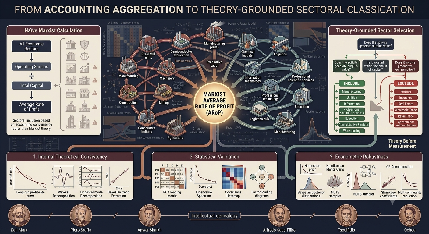
  • Sectorial Exclusion Criteria in the Marxist Analysis of the Average Rate of Profit: The United States Case (1960-2020)

    Sectorial Exclusion Criteria in the Marxist Analysis of the Average Rate of Profit: The United States Case (1960-2020)

    What Counts as “The Economy”? A Marxist Framework for Measuring Capitalism’s Rate of Profit
    Marxist Economics  ·  Econometrics  ·  Political Economy

    What Counts as “The Economy”?
    A Marxist Framework for Measuring Capitalism’s Rate of Profit

    How one researcher built a theoretically rigorous rulebook for a question everyone answers differently — and what happens when you let the data decide for itself.

    In 1984, two economists named Anwar Shaikh and Edgardo Ochoa opened a research tradition that would span four decades: empirically measuring Marx’s most consequential prediction — that capitalism’s average rate of profit tends to fall over time. Since then, dozens of studies have followed, each arriving at the same fundamental calculation, but each choosing differently which sectors of the economy to include. Some count everything. Others exclude finance and government. Still others carve out a narrower productive core. The results? They disagree — sometimes dramatically — about whether the profit rate actually falls.

    The problem isn’t sloppy math. It’s that nobody has ever agreed on a standard for deciding which economic activities belong in the calculation. José Mauricio Gómez Julián’s recent paper aims to change that.

    The Question Nobody Agrees On

    Here’s the issue in plain terms. Suppose you want to calculate the “average rate of profit” for the entire U.S. economy over sixty years. You need two things: the total surplus value produced and the total capital invested. To get these, you aggregate data from individual sectors — agriculture, manufacturing, finance, retail, government, and so on.

    But should finance be in there? Finance doesn’t manufacture anything; it redistributes money. Should government? The government doesn’t compete for profits. Should retail trade? A retailer buys finished goods and sells them at a markup, but Marx argued that the act of buying and selling doesn’t create new value — it merely realizes value already embedded in the commodity.

    These aren’t arbitrary questions. If you include sectors that redistribute value rather than create it, you can artificially inflate or deflate the measured profit rate, potentially masking the very tendency Marx predicted. Different researchers have made different choices, and the field has lacked a unified standard — until this paper.

    Three Pillars: The Theoretical Logic Behind the Criteria

    Gómez Julián’s framework is built on three interlocking concepts from Marx’s political economy. The underlying logic of the entire procedure can be stated simply: an economic sector should be included in the average-rate-of-profit calculation if, and only if, its workforce performs productive labor as Marx defined it — labor that is subordinated to capital and directly produces surplus value, or that constitutes an indispensable material condition for that production to occur. Everything else is excluded.

    Let’s walk through each pillar to see how this logic unfolds in practice.

    1. Productive vs. Unproductive Labor

    The most fundamental distinction in Marx’s economics is between labor that creates value and labor that doesn’t. Productive labor, in the Marxist sense, isn’t about whether work is “useful” in everyday language. It’s a technical category: productive labor is work performed under the subordination of capital that produces surplus value — the unpaid portion of the working day that capitalists appropriate for free.

    Unproductive labor, on the other hand, doesn’t generate new value. It may be socially necessary (think of a cashier or an accountant processing invoices), but it merely facilitates the transfer or realization of value that was already created elsewhere in the production process. It is, as Marx called it, a faux frais — a cost that must be paid out of surplus value rather than one that generates it.

    The mere functions performed by capital in the sphere of circulation — the operations necessary to serve as the vehicle for the metamorphoses of commodity-capital — do not create value or surplus value.

    — Karl Marx, Capital, Volume II

    In other words, the act of buying and selling, however essential for capitalism to function, is not productive in the value-theoretic sense. The merchant who buys goods cheaply and sells them at a markup doesn’t create value through the exchange itself; they merely appropriate a share of value created by productive workers elsewhere.

    2. Location in the Circuit of Capital

    Capital doesn’t just sit still. It moves through a circuit: it begins as commodities filled with freshly produced surplus value (C’), converts into money through sale in the market (M), and then transforms back into new commodities — raw materials, machinery, labor power — to restart production (C → C’). Activities that feed into this productive cycle — that help produce, maintain, or prepare commodities for the next round of production — sit inside the circuit. Activities that operate outside it (like government services aimed at general welfare, or purely redistributive financial operations) sit outside.

    This criterion is critical because it captures something the productive/unproductive distinction alone might miss: even an activity that doesn’t directly produce surplus value can be included if it constitutes an indispensable material precondition for the circuit to continue. Transportation is the classic example — it doesn’t transform a commodity’s physical form, but it physically moves goods to where they’re needed for consumption or further production, which Marx explicitly recognized as a productive act that adds value.

    3. Relationship with Surplus Value

    The final criterion is the most direct: does this activity produce surplus value, or is it an indispensable condition for surplus value production? If it directly creates value through productive labor, include it. If it’s a necessary supporting activity embedded in the productive circuit, include it. If it merely redistributes value already produced, or operates on entirely different logic (like government), exclude it.

    The logic here is that surplus value is the lifeblood of capitalist accumulation. Any sector that doesn’t contribute to its creation or materially enable it is, from the standpoint of the accumulation process, extraneous to the dynamic you’re trying to measure.

    The Service Sector Problem

    One of the paper’s most valuable theoretical contributions is its treatment of services. When Marx wrote, there was no statistical concept of a “service sector.” Modern macroeconomic data lumps together wildly heterogeneous activities under this label — everything from software development to hairdressing to hospital care.

    Gómez Julián, drawing on Tregenna (2009), identifies three types of service activities:

    • Those that directly produce surplus value (e.g., software development subcontracted by a manufacturing firm, transportation of goods)
    • Those that facilitate surplus value production elsewhere (e.g., warehousing that preserves commodity properties, scientific research contracted by industry)
    • Those that remain outside the circuit of capital (e.g., government administration, purely redistributive finance)

    This means you cannot simply include or exclude “services” wholesale. Each activity must be examined on its own terms, disaggregated, and asked: does this particular service perform productive labor, or doesn’t it? For “hybrid” sectors that contain both productive and unproductive components, the researcher must determine the proportions and decide based on which dominates.

    Applying the Criteria: What’s In, What’s Out

    Using Bureau of Economic Analysis data for the United States (1960–2020), Gómez Julián applies these theoretical criteria to 46 consolidated economic sectors. The result is a clear binary classification.

    Included — Productive

    • Farms
    • Forestry, fishing & related activities
    • Oil & gas extraction
    • Mining (except oil & gas)
    • Support activities for mining
    • Utilities
    • Construction
    • All manufacturing (wood, metals, machinery, electronics, motor vehicles, textiles, chemicals, petroleum, paper, printing, plastics, rubber, furniture, food & beverage, apparel, computers, etc.)
    • Transportation
    • Warehousing & storage
    • Information
    • Professional, scientific & technical services
    • Management of companies & enterprises
    • Administrative & waste management services
    • Educational services
    • Arts, entertainment & recreation
    • Accommodation
    • Food services & drinking places
    • Other services (except government)

    Excluded — Non-Productive

    • Wholesale trade
    • Retail trade
    • Finance & insurance
    • Real estate
    • Rental & leasing services
    • Health care & social assistance
    • Federal general government
    • Federal government enterprises
    • State & local general government
    • State & local government enterprises

    Most of these are straightforward once you accept the theoretical framework. Agriculture, mining, manufacturing — clearly productive. Finance, real estate, government — clearly outside the surplus-value production process. But several borderline cases required careful reasoning.

    The Borderline Cases

    Warehousing and storage might seem like a pure logistics function, but the paper argues that preserving the physical properties of commodities before they enter the sphere of circulation is a material precondition for their existence as commodities. Without storage, many goods would deteriorate and lose their use-value. This makes warehousing an indispensable part of the productive process, not merely a cost of circulation.

    Educational services is perhaps the most controversial inclusion. It encompasses private, public, and non-profit components. The classification system doesn’t specify their proportions. But excluding the sector entirely would mean ignoring a fundamental element for reproducing the skilled labor force in a highly industrialized economy — a cost that productive capital must bear one way or another.

    Administrative and waste management services includes activities that generate surplus value (document preparation for productive firms, personnel placement) alongside activities that don’t (security services, household cleaning). The paper argues that since most of the economy consists of productive sectors, and most of these services are contracted by those productive sectors, the productive component likely dominates.

    Information produces and distributes cultural products, software, broadcasting content, and data. In accordance with the criteria — these are material products of creative and technical labor, increasingly subcontracted by productive enterprises — it is included.

    The Econometric Validation: Three Blind Tests

    Here is where the paper’s methodology becomes genuinely innovative. Gómez Julián doesn’t merely propose theoretical criteria and declare victory. He subjects the entire framework to empirical testing using three fundamentally different statistical methods.

    A critical point: These econometric methods operate with zero knowledge of Marxist theory. They do not distinguish between “productive” and “unproductive” labor. They have never heard of the circuit of capital. They simply analyze the raw data for all 47 economic sectors and tell you which ones structurally matter for the economy’s behavior. This makes them a powerful independent test — a way to ask the data itself which sectors form the economy’s real core.

    Test 1: Principal Component Analysis (PCA)

    PCA is a dimensionality reduction technique that identifies the directions (called “principal components”) along which the economy’s sectoral data varies most. Think of it as asking: if the entire economy were a cloud of data points, which directions through that cloud capture the most movement?

    Applied to all 47 sectors simultaneously, PCA found that economic variance is highly concentrated: a small number of sectors drive most of the variation, while many others contribute only marginal noise. Using a rigorous statistical criterion — fitting probability distributions to each sector’s contribution and selecting those in the top decile — PCA identified 26 sectors as structurally significant. A post-hoc validation confirmed that none of the 21 excluded sectors had sufficient statistical weight (eigenvalue exceeding 1) to constitute an independent driver.

    The first principal component was dominated by corporate and financial services. The second by a logistics-industrial chain. The fourth by extractive natural resources. The seventh by education and public administration.

    Test 2: Regularized Horseshoe Regression (RHR)

    This Bayesian method uses a “global-local shrinkage” prior that aggressively compresses noise toward zero while preserving strong signals — think of it as a statistical metal detector that ignores pebbles but rings loudly for gold. The name “Horseshoe” is not a metaphor; it refers to the literal U-shaped geometry of the shrinkage coefficient’s probability distribution, which piles mass at the extremes (fully suppress or fully preserve) rather than settling at mediocre intermediate values like conventional methods.

    Gómez Julián specified the model to predict total gross operating surplus from total variable capital across all sectors — deliberately grounding the specification in the labor theory of value. The severe multicollinearity inherent in input-output data (sectors move together — when steel production grows, automobile production grows) meant that no individual sector achieved traditional statistical significance. This isn’t a failure. As economists Christopher Achen and Olivier Blanchard have argued, multicollinearity in macroeconomic data is not a “problem” to be fixed with clever statistics; it’s an intrinsic, ontological property of how economies work. Blanchard memorably called it “God’s will.”

    What the model could provide was a predictive ranking based on projected predictive density (ELPD): which sectors reduce prediction error fastest. The top 15 sectors identified were:

    1. Retail Trade
    2. Textile Mills & Products
    3. Fabricated Metal Products
    4. Administrative & Waste Management Services
    5. Miscellaneous Manufacturing
    6. Construction
    7. Educational Services
    8. Electrical Equipment, Appliances & Components
    9. Nonmetallic Mineral Products
    10. Support Activities for Mining
    11. Printing & Related Support Activities
    12. Primary Metals
    13. Food Services & Drinking Places
    14. State & Local General Government
    15. Transportation

    Test 3: Dynamic Factor Model (DFM)

    The DFM extracts hidden “latent factors” from the 47 sectoral time series — unobserved forces that cause sectors to move together. The model found two such factors: one capturing short-term cyclical shocks (low persistence, autoregressive coefficient of 0.33) and one carrying the secular, long-term trend (high persistence, autoregressive coefficient of 0.91). These two factors together explain about 34% of total sectoral variation.

    Through an elaborate multi-stage validation involving stability selection, synchronized block bootstrap resampling (300 replications), and a novel “Full-Robust Thresholding” algorithm that generates counterfactual null distributions and corrects for factor indeterminacy via the Hungarian algorithm, the model identified which sectors are most structurally synchronized with these systemic factors.

    The sectors with the highest structural weight were: Real Estate, followed by State & Local General Government and Federal General Government, then Retail Trade and Food Services, with Utilities and Chemical Products providing the industrial baseline.

    The Key Revelation: Theory and Data Diverge

    Now comes the most thought-provoking finding in the paper. The econometric methods — which are purely data-driven and completely agnostic to Marxist theory — identify a set of “core” sectors that overlaps with but also substantially differs from the theoretical classification.

    Where Theory and Data Agree

    Manufacturing sectors (textiles, metals, fabricated products, miscellaneous manufacturing) appear across multiple econometric methods and are unambiguously included by the theoretical criteria.

    Administrative & waste management services ranks 4th in the RHR and is theoretically included as productive.

    Educational services appears in the RHR ranking (7th) and is theoretically included.

    Transportation appears in the RHR ranking (15th) and is theoretically included.

    Construction appears prominently in both RHR (6th) and PCA, and is theoretically included.

    Utilities appear in the DFM results and are theoretically included.

    These convergences suggest that the theoretical criteria are tracking something real in the data: the sectors that Marx identified as productive are indeed among those that structurally drive the economy.

    Where Theory and Data Disagree — And Why It Matters

    Real Estate dominates the DFM results (ranked #1 in structural weight) but is theoretically excluded as non-productive and fictitious.

    Government sectors (federal and state/local) rank among the top DFM sectors but are theoretically excluded because they don’t pursue profit maximization.

    Retail Trade ranks #1 in the RHR and appears prominently in the DFM, yet is theoretically excluded as pure circulation.

    Finance & insurance dominate the first principal component in PCA but are theoretically excluded.

    Health care has the highest eigenvalue among all excluded sectors in PCA’s post-hoc validation table but is theoretically excluded.

    What does this divergence mean? The paper interprets it as profoundly significant. Sectors like real estate, government, and retail trade have “effectively colonized the macro-dynamics of the US rate of profit.” They statistically dominate the national accounting aggregates — they are the forces that shape the observed numbers — even though Marxist theory classifies them as unproductive or revenue-consuming.

    In Marx’s own philosophical vocabulary, the phenomenon (what the data shows on its surface) and the essence (what theory identifies as the true engine of value production) diverge. The sectors driving the observable statistical dynamics are not the same as the sectors that, according to the theory, actually generate surplus value. This is not a refutation of either the theory or the data; it’s an insight into how modern capitalism’s surface appearance differs from its underlying structure — exactly as Marx’s own method predicted it would.

    Does the Rate of Profit Fall?

    With the theoretically selected sectors, all three trend-extraction methods — Daubechies wavelet filters (with 8 vanishing moments at decomposition depth 4), Empirical Mode Decomposition, and the Embedded Hodrick-Prescott filter (implemented within a Bayesian unobserved components model with Gibbs sampling) — produce a clear declining long-term trend in the net average rate of profit over 1960–2020. This is precisely what Marx predicted, and it serves as evidence of the internal consistency of the proposed criteria: the new proposition (the sectoral classification) fits harmoniously within the existing system of Marxist propositions.

    For the econometric criteria, the results are remarkably robust: with the single exception of the Hodrick-Prescott filter under the DFM sector selection, all combinations of econometric sector-selection criteria and filtering methods also produce a declining long-term trend. That means:

    • PCA sectors + Wavelet → declining
    • PCA sectors + EMD → declining
    • PCA sectors + HP → declining
    • RHR sectors + Wavelet → declining
    • RHR sectors + EMD → declining
    • RHR sectors + HP → declining
    • DFM sectors + Wavelet → declining
    • DFM sectors + EMD → declining
    • DFM sectors + HP → not clearly declining

    Regardless of which sectors you choose — based on careful Marxist reasoning or on pure data analysis — and regardless of which statistical filter you use, the long-term profit rate falls. The HP-DFM exception is attributed to the filter’s parametric specifications (its linear structure and second-order Markov assumption for the trend) potentially interacting poorly with a sectoral composition heavily weighted toward government and real estate — sectors whose dynamics may follow different logics than productive capital.

    The Empirical Mode Decomposition, being a non-parametric technique that adapts to the data’s intrinsic patterns without imposing prior assumptions about functional form, consistently produced the most accentuated declining trend across all sector selections.

    Why This Paper Matters

    Gómez Julián’s work makes three contributions that will resonate well beyond the boundaries of Marxist economics:

    First, methodological standardization. For the first time, there is a theoretically grounded, explicit, and reproducible set of criteria for deciding which sectors belong in Marxist profit-rate calculations. This addresses a four-decade-old methodological gap and enables meaningful comparison across future studies. Researchers can now reproduce the same classification, apply it to different countries or time periods, and test whether the declining tendency holds universally.

    Second, the theory-data tension as an analytical asset. Rather than hiding the divergence between theoretical classifications and empirical results, the paper treats it as a finding in its own right. The fact that unproductive sectors statistically dominate the macro-dynamics of the profit rate tells us something important about how modern capitalism appears on its surface versus how it functions at its core. It demonstrates, empirically, that Marx’s concept of “essence” and “phenomenon” isn’t merely philosophical abstraction — it describes a real, measurable gap in economic data.

    Third, the robustness of the declining trend. Whether you select sectors based on careful Marxist reasoning or let unsupervised statistical methods decide for you, the long-term profit rate declines. This convergence across radically different methodologies strengthens the empirical case for what may be Marx’s most famous — and most contested — prediction.

    The paper does not claim to have proven Marx right beyond doubt. Internal consistency, it notes, does not guarantee overall theoretical validity. But it has demonstrated that when you take the theory seriously — when you build your measurement instrument to match the conceptual categories rather than stuffing everything into the equation and hoping for the best — the data speaks in a direction that Marx would have recognized.