

Espartaco

“Is that to say we are against Free Trade? No, we are for Free Trade, because by Free Trade all economical laws, with their most astounding contradictions, will act upon a larger scale, upon the territory of the whole earth; and because from the uniting of all these contradictions in a single group, where they will stand face to face, will result the struggle which will itself eventuate in the emancipation of the proletariat.”

Karl Heinrich Marx · Marx-Engels Collected Works, Vol. VI, p. 290

EnglishEspañol

Tag: econometric methods

  • valueprhr: When Do Market Prices Reflect the Labor That Produced Them? A Modern R Toolkit for an Old Question

    valueprhr: When Do Market Prices Reflect the Labor That Produced Them? A Modern R Toolkit for an Old Question

    You can also find this library at CRAN and download it directly from R and RStudio.

    An introduction to an R package that brings Bayesian inference, panel data econometrics, and rigorous validation to one of political economy’s most enduring empirical debates.


    Why This Package Exists

    Here is a question that has occupied economists for over two centuries: when you pay for something, does the price you pay bear any systematic relationship to the labor required to make it?

    Adam Smith thought so. David Ricardo refined the idea. Karl Marx built an entire theory of exploitation on it. And since the mid-twentieth century, empirical researchers have been trying to measure the strength of this correspondence with real-world data.

    The challenge has always been methodological. The datasets are panel data — prices observed across many economic sectors over many time periods — and they demand techniques that respect both the cross-sectional structure (different industries behave differently) and the temporal dimension (relationships can shift over time). A simple scatterplot of values against prices, however illustrative, will not settle the question.

    valueprhr is an R package built to close this methodological gap. It provides a complete, reproducible pipeline: from raw price matrices to model estimation, from Bayesian inference to out-of-sample validation, from structural break detection to side-by-side model comparison. It was designed for political economy, but as we will see, its toolkit applies to any panel data problem where you need to assess the correspondence between two variables across entities and time.


    The Core Idea (in Plain Language)

    In the classical and Marxian tradition, the value of a commodity is determined by the total labor time — direct and indirect — required to produce it. If a table requires 10 hours of socially necessary labor and a chair requires 5, the table’s value is twice the chair’s.

    This gives rise to what economists call direct prices (denoted pd): prices that are strictly proportional to the labor embodied in each commodity. They represent what prices would be if they perfectly mirrored labor content.

    But capitalism does not work that way. Capital flows between sectors seeking the highest return, and competition tends to equalize the rate of profit across industries. The prices that emerge from this process are called prices of production (denoted pπ). They redistribute surplus value: sectors with higher organic composition of capital (more machinery relative to labor) tend to have prices of production above their direct prices, and vice versa.

    The central empirical question is: despite this redistribution, how closely do direct prices and prices of production correspond?

    The standard test is a log-linear regression:

    ln(pπit) = α + β · ln(pdit) + uit

    where i indexes sectors and t indexes time periods.

    Three hypotheses are at stake:

    • β ≈ 1: a one-percent increase in direct prices is associated with roughly a one-percent increase in production prices (proportionality).
    • R² ≈ 1: direct prices explain the vast majority of the variation in production prices.
    • Stability: the relationship holds consistently across time periods.

    If all three hold, the labor theory of value has strong empirical support. valueprhr gives you the tools to test each one rigorously.


    What’s Inside the Package

    valueprhr organizes its functionality into six modules. Here is what each does and why it matters.

    1. Data Preparation

    Real-world data rarely arrives in the format econometric methods require. The package accepts two data frames in wide format (rows = years, columns = sectors) — one for direct prices, one for production prices — and converts them into the long-format panel structure that econometric models expect.

    library(valueprhr)
    # Wide format: Year | Agriculture | Manufacturing | Mining | ...
    direct <- read.csv("direct_prices.csv")
    production <- read.csv("production_prices.csv")
    # Convert to long panel: Year, Sector, direct, production, log_direct, log_production
    panel <- prepare_panel_data(direct, production, log_transform = TRUE)
    head(panel)
    #> Year Sector direct production log_direct log_production
    #> 1 1960 Agriculture 45.2 48.1 3.81 3.87
    #> 2 1961 Agriculture 46.0 49.0 3.83 3.89
    #> ...

    The function prepare_log_matrices() does the same job but returns matrix format, which is what the multivariate methods (PLS, CCA) need.

    2. Panel Data Models

    This is where the core econometrics happens. The package implements two complementary specifications:

    Two-Way Fixed Effects (FE) controls for both sector-specific and time-specific unobserved heterogeneity:

    Yit = αi + γt + β · Xit + εit

    In plain terms: every sector has its own baseline (some sectors are systematically more expensive), every year has its own macroeconomic conditions (inflation, crises), and the model isolates the within variation to estimate the core relationship.

    fe <- fit_twoway_fe(panel, robust_se = TRUE, cluster_type = "group")
    print(fe)
    #> Two-Way Fixed Effects Model
    #> ============================
    #> Observations: 1200 | Sectors: 20 | Years: 60
    #> R-squared: 0.9876 | Adjusted R-squared: 0.9870
    #>
    #> log_direct coefficient:
    #> Estimate = 0.9754, SE = 0.0123, t = 79.30, p = 0.0000

    The cluster_type = "group" option computes cluster-robust standard errors at the sector level, which accounts for serial correlation within each sector’s time series.

    Mundlak Correlated Random Effects (CRE) takes a different route. Instead of dummy variables for every sector, it decomposes the predictor into a within-sector component (how Xit deviates from sector i‘s average) and a between-sector component (the sector average itself):

    Yit = α + βW · (Xiti) + βB · i + ui + εit

    In data science language: this is a way to control for group-level confounders without the computational cost of N dummy variables. If βW = βB, the within and between effects are the same, and a simpler Random Effects model suffices. If they differ, the relationship between values and prices operates differently within a sector over time than across sectors.

    # Add Mundlak terms
    panel_cre <- create_mundlak_data(panel, x_var = "log_direct")
    # Fit the model
    cre <- fit_mundlak_cre(panel_cre, include_time_fe = TRUE)
    print(cre)
    #> Mundlak Correlated Random Effects Model
    #> =========================================
    #> Within-sector effect (beta_W): 0.9680
    #> Between-sector effect (beta_B): 0.9912
    #>
    #> Mundlak test H0: beta_W = beta_B
    #> F-stat = 2.14, p-value = 0.1438
    #> -> Fail to reject H0: RE/CRE specification is consistent

    The function test_mundlak_specification() formalizes this check. A low p-value means you should stick with Fixed Effects; a high p-value means the simpler model is adequate.

    The package also includes a Panel Granger Causality test (the Dumitrescu-Hurlin procedure), which tests whether past values of direct prices help predict current production prices — and vice versa.

    panel_granger_test(panel, lags = c(1, 2))
    #> direction lag W_stat Z_stat p_value significant
    #> 1 direct -> production 1 8.432 3.126 0.0018 TRUE
    #> 2 direct -> production 2 6.215 2.441 0.0146 TRUE
    #> 3 production -> direct 1 5.890 2.103 0.0354 TRUE
    #> 4 production -> direct 2 4.012 1.332 0.1828 FALSE

    3. Bayesian Models

    Classical (frequentist) estimation gives you a single point estimate for β. Bayesian methods give you a full probability distribution over possible values, incorporating your prior beliefs and updating them with the data.

    In econometric language: instead of β̂ = 0.975 ± 0.012, you get a posterior distribution showing that β lies between 0.95 and 1.00 with 95% probability.

    The package offers two Bayesian approaches:

    Sector-by-Sector Bayesian GLM fits an independent Bayesian linear model for each sector, using weakly informative priors (the rstanarm package handles the MCMC sampling via Stan). Each sector gets its own slope and intercept, along with Leave-One-Out Cross-Validation (LOO-CV) scores.

    bayes <- fit_bayesian_glm_sectors(
    direct, production,
    chains = 4, iter = 4000
    )
    print(bayes$summary_table)
    #> Sector beta_mean beta_sd beta_lower beta_upper elpd looic n_obs
    #> 1 Agriculture 0.982 0.025 0.933 1.031 -42.3 84.6 60
    #> 2 Manufacturing 0.971 0.031 0.910 1.031 -38.7 77.4 60
    #> 3 Mining 0.958 0.042 0.876 1.041 -45.1 90.2 60
    #> ...

    In data science language: LOO-CV is a principled way to assess out-of-sample predictive performance without holding out data. The LOOIC (LOO Information Criterion) is the Bayesian analogue of AIC — lower is better.

    Bayesian Hierarchical Model goes further by pooling information across sectors. Instead of treating each sector in isolation, it assumes that sector-specific slopes are drawn from a common population distribution:

    βi ~ N(μβ, σβ2)

    Sectors with less data “borrow strength” from the population mean. This is especially valuable when some sectors have short time series.

    hier <- fit_bayesian_hierarchical(panel, include_time = TRUE)
    print(hier)
    #> Bayesian Hierarchical Model
    #> ============================
    #> Observations: 1200 | Sectors: 20
    #>
    #> LOO-CV:
    #> ELPD = -312.45
    #> LOOIC = 624.90
    #>
    #> Population-level effects:
    #> parameter mean sd 2.5% 97.5%
    #> 1 (Intercept) 0.1423 0.0892 -0.032 0.317
    #> 2 log_direct 0.9734 0.0145 0.945 1.002
    #> 3 Time_scaled 0.0031 0.0018 -0.0004 0.007

    4. Multivariate Analysis

    When the number of sectors (N) is large relative to the number of time periods (T), standard regression becomes unstable. This is the “small T, large N” problem common in panel data. The package offers three multivariate techniques to handle it:

    Partial Least Squares (PLS) extracts latent components that explain covariance between direct prices and production prices. It handles multicollinearity gracefully and is widely used in chemometrics, genomics, and now in value-price analysis.

    matrices <- prepare_log_matrices(direct, production)
    pls <- fit_pls_multivariate(
    matrices$X_clean, matrices$Y_clean,
    max_components = 8
    )
    print(pls)
    #> Partial Least Squares (PLS) Regression
    #> =======================================
    #> Optimal components: 3
    #>
    #> R-squared by component:
    #> n_components R2_train R2_cv
    #> 1 1 0.942 0.938
    #> 2 2 0.971 0.965
    #> 3 3 0.984 0.980

    Canonical Correlation Analysis (CCA) finds linear combinations of direct prices and production prices that are maximally correlated. In econometric language: CCA extracts the “shared economic signal” — the common factor driving both sets of prices.

    cca <- run_sparse_cca(matrices$X_clean, matrices$Y_clean, n_components = 3)
    print(cca)
    #> Canonical Correlation Analysis
    #> ===============================
    #> Components: 3
    #>
    #> Canonical correlations:
    #> CC1: r = 0.9987 (Var X: 92.3%, Var Y: 91.8%)
    #> CC2: r = 0.9841 (Var X: 5.1%, Var Y: 5.4%)
    #> CC3: r = 0.9523 (Var X: 1.8%, Var Y: 1.9%)

    The first canonical correlation above 0.99 indicates an extremely tight structural link between the two price systems.

    Panel VAR captures dynamic feedback: do lagged values of direct prices predict current production prices, and vice versa?

    pvar <- fit_panel_var(panel, lags = 2, transformation = "fd")

    5. Cross-Validation

    Standard k-fold cross-validation violates temporal ordering. If you train on 1960–1990 and test on 1985–1990, future information leaks into the training set. The package implements two time-aware approaches:

    Rolling Window CV trains on t₀ … tW, tests on tW+1tW+H, then rolls the window forward.

    cv <- rolling_window_cv(
    panel,
    window_sizes = c(20, 30),
    step_size = 2,
    test_horizon = 3
    )
    print(cv$summary)

    Leave-One-Sector-Out (LOSO) trains on all sectors except one and predicts the held-out sector. This tests cross-sectional generalization: does the value-price relationship estimated from other sectors hold for agriculture? For mining? For finance?

    loso <- leave_one_sector_out(panel)
    print(loso$summary)
    #> metric mean sd
    #> 1 RMSE 0.04521 0.01832
    #> 2 MAE 0.03587 0.01456
    #> 3 R_squared 0.96120 0.02340

    An average R² above 0.96 in LOSO-CV means the relationship generalizes robustly across sectors.

    6. Structural Break Tests

    Has the value-price relationship been stable over time? Or did it shift at some point — due to globalization, a methodological change in data construction, a technological revolution, or a regime shift in profit rate equalization?

    The package aggregates the panel to a time series and applies a battery of tests:

    breaks <- test_structural_breaks(panel, break_date = 1990)
    print(breaks)
    #> Structural Break Tests
    #> ========================
    #> Time-series observations: 60
    #>
    #> Chow Test:
    #> Break date: 1990
    #> F-stat = 1.8420, p = 0.1687
    #>
    #> supF / Bai-Perron Test:
    #> supF = 5.2130, p = 0.0842
    #> Breaks detected: 0

    A non-significant result is actually good news here: it means the value-price correspondence has been structurally stable across the entire sample period.


    The Full Pipeline in One Command

    If you want to run everything at once — data preparation, FE and CRE models, cross-validation, structural break tests, and model comparison — the package offers a single entry point:

    results <- run_full_analysis(
    direct,
    production,
    run_bayesian = FALSE, # Set TRUE if you have rstanarm installed
    run_cv = TRUE,
    run_breaks = TRUE,
    verbose = TRUE
    )
    # Access everything
    print(results$comparison)
    print(results$cv_summary)
    cat(format_break_results(results$breaks))

    You can then export the comparison table and CV results to CSV:

    export_results_csv(
    results$comparison,
    results$cv_summary,
    output_dir = "results/"
    )

    Beyond Political Economy: General Panel Data Applications

    Although valueprhr was built for the specific question of value-price correspondence, its methods are general-purpose panel data tools. Any research problem involving the relationship between two variables observed across entities and time can benefit from the package:

    • Health economics: Does out-of-pocket spending track underlying treatment costs across regions over time?
    • Environmental economics: Do carbon prices reflect the embodied emissions of goods across industries?
    • Education: Do standardized test scores correspond to instructional expenditure across school districts over decades?
    • Finance: Do book values predict market valuations across sectors?
    • Any two-variable panel regression where you need fixed effects, Mundlak decomposition, robust standard errors, time-aware cross-validation, or structural break detection.

    The key requirement is that your data has a panel structure (entities × time) and that the distributional assumptions of the models are reasonable for your context. The methods — two-way FE, Mundlak CRE, Bayesian hierarchical models, PLS, CCA, rolling-window CV, structural break tests — are econometric staples that transcend any particular application domain.


    Installation and Dependencies

    The package requires R ≥ 4.1.0. Core functionality depends only on base R and the Metrics package. Extended features (Bayesian models, panel data infrastructure, structural break tests) are handled through soft dependencies that are loaded on demand:

    # Install from GitHub
    install.packages("devtools")
    devtools::install_github("isadorenabi/valueprhr")
    # Optional: install all suggested packages at once
    suggested <- c(
    "rstanarm", "loo", "plm", "lme4", "pls", "vars",
    "panelvar", "strucchange", "lmtest", "sandwich",
    "dplyr", "tidyr", "tibble"
    )
    install.packages(suggested[!sapply(suggested, requireNamespace, quietly = TRUE)])

    Note for Bayesian models: rstanarm requires a working C++ toolchain — Rtools on Windows, Xcode Command Line Tools on macOS, or build-essential on Linux.


    What Makes This Package Methodologically Different

    Three features distinguish valueprhr from a hand-rolled analysis:

    1. Time-aware validation. Most applied work reports in-sample R² as evidence of fit. valueprhr pairs every model with rolling-window and leave-one-sector-out cross-validation, giving you out-of-sample performance that is honest about temporal dependence and cross-sectional generalization.
    2. The Mundlak decomposition. By splitting effects into within-sector and between-sector components, the package lets you test whether the value-price relationship operates at the sector level (structural), at the temporal level (cyclical), or both. This is a nuance that most empirical studies in this literature overlook.
    3. Bayesian hierarchical pooling. Sectors with short time series are a common headache. The hierarchical model lets small sectors borrow statistical strength from the population, producing more stable estimates than independent sector-by-sector regressions.

    A Note on the Underlying Data

    The wiki documentation mentions that market price indices used in this framework are constructed by temporally disaggregating the aggregate Consumer Price Index using the Input-Output matrix as a structural indicator, relying on closed-form Bayesian solutions from the BayesianDisaggregation library. This is a methodological detail worth understanding: the sectoral prices are not raw market quotes but statistically consistent decompositions of the macroeconomic aggregate. This ensures that the estimated sectoral price movements add up to the observed CPI, a property that many ad hoc sectoral price datasets lack.


    Citation

    If you use valueprhr in your research:

    @software{gomezjulian2025valueprhr,
    author = {Gómez Julián, José Mauricio},
    title = {valueprhr: Value-Price Analysis with Bayesian and Panel Data Methods},
    year = {2025},
    url = {https://github.com/isadorenabi/valueprhr},
    note = {R package version 0.1.0}
    }

    Author: José Mauricio Gómez Julián — ORCID — isadore.nabi@pm.me

    License: MIT

    Repository: github.com/IsadoreNabi/valueprhr


    The labor theory of value is either one of the most important ideas in the history of economics or one of the most contested. Either way, it deserves better tools than a spreadsheet and a prayer. valueprhr brings the full machinery of modern econometrics to the question — and lets the data speak for itself.
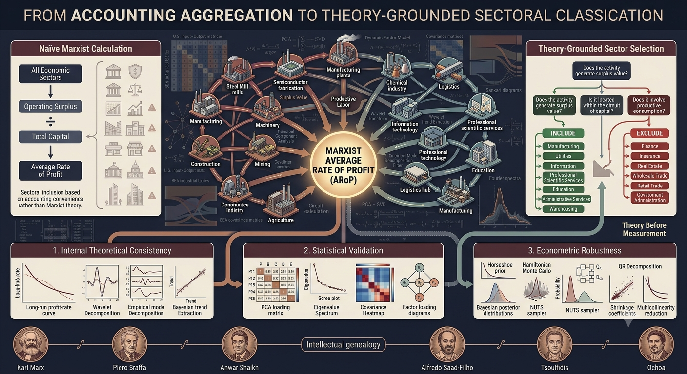
  • Sectorial Exclusion Criteria in the Marxist Analysis of the Average Rate of Profit: The United States Case (1960-2020)

    Sectorial Exclusion Criteria in the Marxist Analysis of the Average Rate of Profit: The United States Case (1960-2020)

    What Counts as “The Economy”? A Marxist Framework for Measuring Capitalism’s Rate of Profit
    Marxist Economics  ·  Econometrics  ·  Political Economy

    What Counts as “The Economy”?
    A Marxist Framework for Measuring Capitalism’s Rate of Profit

    How one researcher built a theoretically rigorous rulebook for a question everyone answers differently — and what happens when you let the data decide for itself.

    In 1984, two economists named Anwar Shaikh and Edgardo Ochoa opened a research tradition that would span four decades: empirically measuring Marx’s most consequential prediction — that capitalism’s average rate of profit tends to fall over time. Since then, dozens of studies have followed, each arriving at the same fundamental calculation, but each choosing differently which sectors of the economy to include. Some count everything. Others exclude finance and government. Still others carve out a narrower productive core. The results? They disagree — sometimes dramatically — about whether the profit rate actually falls.

    The problem isn’t sloppy math. It’s that nobody has ever agreed on a standard for deciding which economic activities belong in the calculation. José Mauricio Gómez Julián’s recent paper aims to change that.

    The Question Nobody Agrees On

    Here’s the issue in plain terms. Suppose you want to calculate the “average rate of profit” for the entire U.S. economy over sixty years. You need two things: the total surplus value produced and the total capital invested. To get these, you aggregate data from individual sectors — agriculture, manufacturing, finance, retail, government, and so on.

    But should finance be in there? Finance doesn’t manufacture anything; it redistributes money. Should government? The government doesn’t compete for profits. Should retail trade? A retailer buys finished goods and sells them at a markup, but Marx argued that the act of buying and selling doesn’t create new value — it merely realizes value already embedded in the commodity.

    These aren’t arbitrary questions. If you include sectors that redistribute value rather than create it, you can artificially inflate or deflate the measured profit rate, potentially masking the very tendency Marx predicted. Different researchers have made different choices, and the field has lacked a unified standard — until this paper.

    Three Pillars: The Theoretical Logic Behind the Criteria

    Gómez Julián’s framework is built on three interlocking concepts from Marx’s political economy. The underlying logic of the entire procedure can be stated simply: an economic sector should be included in the average-rate-of-profit calculation if, and only if, its workforce performs productive labor as Marx defined it — labor that is subordinated to capital and directly produces surplus value, or that constitutes an indispensable material condition for that production to occur. Everything else is excluded.

    Let’s walk through each pillar to see how this logic unfolds in practice.

    1. Productive vs. Unproductive Labor

    The most fundamental distinction in Marx’s economics is between labor that creates value and labor that doesn’t. Productive labor, in the Marxist sense, isn’t about whether work is “useful” in everyday language. It’s a technical category: productive labor is work performed under the subordination of capital that produces surplus value — the unpaid portion of the working day that capitalists appropriate for free.

    Unproductive labor, on the other hand, doesn’t generate new value. It may be socially necessary (think of a cashier or an accountant processing invoices), but it merely facilitates the transfer or realization of value that was already created elsewhere in the production process. It is, as Marx called it, a faux frais — a cost that must be paid out of surplus value rather than one that generates it.

    The mere functions performed by capital in the sphere of circulation — the operations necessary to serve as the vehicle for the metamorphoses of commodity-capital — do not create value or surplus value.

    — Karl Marx, Capital, Volume II

    In other words, the act of buying and selling, however essential for capitalism to function, is not productive in the value-theoretic sense. The merchant who buys goods cheaply and sells them at a markup doesn’t create value through the exchange itself; they merely appropriate a share of value created by productive workers elsewhere.

    2. Location in the Circuit of Capital

    Capital doesn’t just sit still. It moves through a circuit: it begins as commodities filled with freshly produced surplus value (C’), converts into money through sale in the market (M), and then transforms back into new commodities — raw materials, machinery, labor power — to restart production (C → C’). Activities that feed into this productive cycle — that help produce, maintain, or prepare commodities for the next round of production — sit inside the circuit. Activities that operate outside it (like government services aimed at general welfare, or purely redistributive financial operations) sit outside.

    This criterion is critical because it captures something the productive/unproductive distinction alone might miss: even an activity that doesn’t directly produce surplus value can be included if it constitutes an indispensable material precondition for the circuit to continue. Transportation is the classic example — it doesn’t transform a commodity’s physical form, but it physically moves goods to where they’re needed for consumption or further production, which Marx explicitly recognized as a productive act that adds value.

    3. Relationship with Surplus Value

    The final criterion is the most direct: does this activity produce surplus value, or is it an indispensable condition for surplus value production? If it directly creates value through productive labor, include it. If it’s a necessary supporting activity embedded in the productive circuit, include it. If it merely redistributes value already produced, or operates on entirely different logic (like government), exclude it.

    The logic here is that surplus value is the lifeblood of capitalist accumulation. Any sector that doesn’t contribute to its creation or materially enable it is, from the standpoint of the accumulation process, extraneous to the dynamic you’re trying to measure.

    The Service Sector Problem

    One of the paper’s most valuable theoretical contributions is its treatment of services. When Marx wrote, there was no statistical concept of a “service sector.” Modern macroeconomic data lumps together wildly heterogeneous activities under this label — everything from software development to hairdressing to hospital care.

    Gómez Julián, drawing on Tregenna (2009), identifies three types of service activities:

    • Those that directly produce surplus value (e.g., software development subcontracted by a manufacturing firm, transportation of goods)
    • Those that facilitate surplus value production elsewhere (e.g., warehousing that preserves commodity properties, scientific research contracted by industry)
    • Those that remain outside the circuit of capital (e.g., government administration, purely redistributive finance)

    This means you cannot simply include or exclude “services” wholesale. Each activity must be examined on its own terms, disaggregated, and asked: does this particular service perform productive labor, or doesn’t it? For “hybrid” sectors that contain both productive and unproductive components, the researcher must determine the proportions and decide based on which dominates.

    Applying the Criteria: What’s In, What’s Out

    Using Bureau of Economic Analysis data for the United States (1960–2020), Gómez Julián applies these theoretical criteria to 46 consolidated economic sectors. The result is a clear binary classification.

    Included — Productive

    • Farms
    • Forestry, fishing & related activities
    • Oil & gas extraction
    • Mining (except oil & gas)
    • Support activities for mining
    • Utilities
    • Construction
    • All manufacturing (wood, metals, machinery, electronics, motor vehicles, textiles, chemicals, petroleum, paper, printing, plastics, rubber, furniture, food & beverage, apparel, computers, etc.)
    • Transportation
    • Warehousing & storage
    • Information
    • Professional, scientific & technical services
    • Management of companies & enterprises
    • Administrative & waste management services
    • Educational services
    • Arts, entertainment & recreation
    • Accommodation
    • Food services & drinking places
    • Other services (except government)

    Excluded — Non-Productive

    • Wholesale trade
    • Retail trade
    • Finance & insurance
    • Real estate
    • Rental & leasing services
    • Health care & social assistance
    • Federal general government
    • Federal government enterprises
    • State & local general government
    • State & local government enterprises

    Most of these are straightforward once you accept the theoretical framework. Agriculture, mining, manufacturing — clearly productive. Finance, real estate, government — clearly outside the surplus-value production process. But several borderline cases required careful reasoning.

    The Borderline Cases

    Warehousing and storage might seem like a pure logistics function, but the paper argues that preserving the physical properties of commodities before they enter the sphere of circulation is a material precondition for their existence as commodities. Without storage, many goods would deteriorate and lose their use-value. This makes warehousing an indispensable part of the productive process, not merely a cost of circulation.

    Educational services is perhaps the most controversial inclusion. It encompasses private, public, and non-profit components. The classification system doesn’t specify their proportions. But excluding the sector entirely would mean ignoring a fundamental element for reproducing the skilled labor force in a highly industrialized economy — a cost that productive capital must bear one way or another.

    Administrative and waste management services includes activities that generate surplus value (document preparation for productive firms, personnel placement) alongside activities that don’t (security services, household cleaning). The paper argues that since most of the economy consists of productive sectors, and most of these services are contracted by those productive sectors, the productive component likely dominates.

    Information produces and distributes cultural products, software, broadcasting content, and data. In accordance with the criteria — these are material products of creative and technical labor, increasingly subcontracted by productive enterprises — it is included.

    The Econometric Validation: Three Blind Tests

    Here is where the paper’s methodology becomes genuinely innovative. Gómez Julián doesn’t merely propose theoretical criteria and declare victory. He subjects the entire framework to empirical testing using three fundamentally different statistical methods.

    A critical point: These econometric methods operate with zero knowledge of Marxist theory. They do not distinguish between “productive” and “unproductive” labor. They have never heard of the circuit of capital. They simply analyze the raw data for all 47 economic sectors and tell you which ones structurally matter for the economy’s behavior. This makes them a powerful independent test — a way to ask the data itself which sectors form the economy’s real core.

    Test 1: Principal Component Analysis (PCA)

    PCA is a dimensionality reduction technique that identifies the directions (called “principal components”) along which the economy’s sectoral data varies most. Think of it as asking: if the entire economy were a cloud of data points, which directions through that cloud capture the most movement?

    Applied to all 47 sectors simultaneously, PCA found that economic variance is highly concentrated: a small number of sectors drive most of the variation, while many others contribute only marginal noise. Using a rigorous statistical criterion — fitting probability distributions to each sector’s contribution and selecting those in the top decile — PCA identified 26 sectors as structurally significant. A post-hoc validation confirmed that none of the 21 excluded sectors had sufficient statistical weight (eigenvalue exceeding 1) to constitute an independent driver.

    The first principal component was dominated by corporate and financial services. The second by a logistics-industrial chain. The fourth by extractive natural resources. The seventh by education and public administration.

    Test 2: Regularized Horseshoe Regression (RHR)

    This Bayesian method uses a “global-local shrinkage” prior that aggressively compresses noise toward zero while preserving strong signals — think of it as a statistical metal detector that ignores pebbles but rings loudly for gold. The name “Horseshoe” is not a metaphor; it refers to the literal U-shaped geometry of the shrinkage coefficient’s probability distribution, which piles mass at the extremes (fully suppress or fully preserve) rather than settling at mediocre intermediate values like conventional methods.

    Gómez Julián specified the model to predict total gross operating surplus from total variable capital across all sectors — deliberately grounding the specification in the labor theory of value. The severe multicollinearity inherent in input-output data (sectors move together — when steel production grows, automobile production grows) meant that no individual sector achieved traditional statistical significance. This isn’t a failure. As economists Christopher Achen and Olivier Blanchard have argued, multicollinearity in macroeconomic data is not a “problem” to be fixed with clever statistics; it’s an intrinsic, ontological property of how economies work. Blanchard memorably called it “God’s will.”

    What the model could provide was a predictive ranking based on projected predictive density (ELPD): which sectors reduce prediction error fastest. The top 15 sectors identified were:

    1. Retail Trade
    2. Textile Mills & Products
    3. Fabricated Metal Products
    4. Administrative & Waste Management Services
    5. Miscellaneous Manufacturing
    6. Construction
    7. Educational Services
    8. Electrical Equipment, Appliances & Components
    9. Nonmetallic Mineral Products
    10. Support Activities for Mining
    11. Printing & Related Support Activities
    12. Primary Metals
    13. Food Services & Drinking Places
    14. State & Local General Government
    15. Transportation

    Test 3: Dynamic Factor Model (DFM)

    The DFM extracts hidden “latent factors” from the 47 sectoral time series — unobserved forces that cause sectors to move together. The model found two such factors: one capturing short-term cyclical shocks (low persistence, autoregressive coefficient of 0.33) and one carrying the secular, long-term trend (high persistence, autoregressive coefficient of 0.91). These two factors together explain about 34% of total sectoral variation.

    Through an elaborate multi-stage validation involving stability selection, synchronized block bootstrap resampling (300 replications), and a novel “Full-Robust Thresholding” algorithm that generates counterfactual null distributions and corrects for factor indeterminacy via the Hungarian algorithm, the model identified which sectors are most structurally synchronized with these systemic factors.

    The sectors with the highest structural weight were: Real Estate, followed by State & Local General Government and Federal General Government, then Retail Trade and Food Services, with Utilities and Chemical Products providing the industrial baseline.

    The Key Revelation: Theory and Data Diverge

    Now comes the most thought-provoking finding in the paper. The econometric methods — which are purely data-driven and completely agnostic to Marxist theory — identify a set of “core” sectors that overlaps with but also substantially differs from the theoretical classification.

    Where Theory and Data Agree

    Manufacturing sectors (textiles, metals, fabricated products, miscellaneous manufacturing) appear across multiple econometric methods and are unambiguously included by the theoretical criteria.

    Administrative & waste management services ranks 4th in the RHR and is theoretically included as productive.

    Educational services appears in the RHR ranking (7th) and is theoretically included.

    Transportation appears in the RHR ranking (15th) and is theoretically included.

    Construction appears prominently in both RHR (6th) and PCA, and is theoretically included.

    Utilities appear in the DFM results and are theoretically included.

    These convergences suggest that the theoretical criteria are tracking something real in the data: the sectors that Marx identified as productive are indeed among those that structurally drive the economy.

    Where Theory and Data Disagree — And Why It Matters

    Real Estate dominates the DFM results (ranked #1 in structural weight) but is theoretically excluded as non-productive and fictitious.

    Government sectors (federal and state/local) rank among the top DFM sectors but are theoretically excluded because they don’t pursue profit maximization.

    Retail Trade ranks #1 in the RHR and appears prominently in the DFM, yet is theoretically excluded as pure circulation.

    Finance & insurance dominate the first principal component in PCA but are theoretically excluded.

    Health care has the highest eigenvalue among all excluded sectors in PCA’s post-hoc validation table but is theoretically excluded.

    What does this divergence mean? The paper interprets it as profoundly significant. Sectors like real estate, government, and retail trade have “effectively colonized the macro-dynamics of the US rate of profit.” They statistically dominate the national accounting aggregates — they are the forces that shape the observed numbers — even though Marxist theory classifies them as unproductive or revenue-consuming.

    In Marx’s own philosophical vocabulary, the phenomenon (what the data shows on its surface) and the essence (what theory identifies as the true engine of value production) diverge. The sectors driving the observable statistical dynamics are not the same as the sectors that, according to the theory, actually generate surplus value. This is not a refutation of either the theory or the data; it’s an insight into how modern capitalism’s surface appearance differs from its underlying structure — exactly as Marx’s own method predicted it would.

    Does the Rate of Profit Fall?

    With the theoretically selected sectors, all three trend-extraction methods — Daubechies wavelet filters (with 8 vanishing moments at decomposition depth 4), Empirical Mode Decomposition, and the Embedded Hodrick-Prescott filter (implemented within a Bayesian unobserved components model with Gibbs sampling) — produce a clear declining long-term trend in the net average rate of profit over 1960–2020. This is precisely what Marx predicted, and it serves as evidence of the internal consistency of the proposed criteria: the new proposition (the sectoral classification) fits harmoniously within the existing system of Marxist propositions.

    For the econometric criteria, the results are remarkably robust: with the single exception of the Hodrick-Prescott filter under the DFM sector selection, all combinations of econometric sector-selection criteria and filtering methods also produce a declining long-term trend. That means:

    • PCA sectors + Wavelet → declining
    • PCA sectors + EMD → declining
    • PCA sectors + HP → declining
    • RHR sectors + Wavelet → declining
    • RHR sectors + EMD → declining
    • RHR sectors + HP → declining
    • DFM sectors + Wavelet → declining
    • DFM sectors + EMD → declining
    • DFM sectors + HP → not clearly declining

    Regardless of which sectors you choose — based on careful Marxist reasoning or on pure data analysis — and regardless of which statistical filter you use, the long-term profit rate falls. The HP-DFM exception is attributed to the filter’s parametric specifications (its linear structure and second-order Markov assumption for the trend) potentially interacting poorly with a sectoral composition heavily weighted toward government and real estate — sectors whose dynamics may follow different logics than productive capital.

    The Empirical Mode Decomposition, being a non-parametric technique that adapts to the data’s intrinsic patterns without imposing prior assumptions about functional form, consistently produced the most accentuated declining trend across all sector selections.

    Why This Paper Matters

    Gómez Julián’s work makes three contributions that will resonate well beyond the boundaries of Marxist economics:

    First, methodological standardization. For the first time, there is a theoretically grounded, explicit, and reproducible set of criteria for deciding which sectors belong in Marxist profit-rate calculations. This addresses a four-decade-old methodological gap and enables meaningful comparison across future studies. Researchers can now reproduce the same classification, apply it to different countries or time periods, and test whether the declining tendency holds universally.

    Second, the theory-data tension as an analytical asset. Rather than hiding the divergence between theoretical classifications and empirical results, the paper treats it as a finding in its own right. The fact that unproductive sectors statistically dominate the macro-dynamics of the profit rate tells us something important about how modern capitalism appears on its surface versus how it functions at its core. It demonstrates, empirically, that Marx’s concept of “essence” and “phenomenon” isn’t merely philosophical abstraction — it describes a real, measurable gap in economic data.

    Third, the robustness of the declining trend. Whether you select sectors based on careful Marxist reasoning or let unsupervised statistical methods decide for you, the long-term profit rate declines. This convergence across radically different methodologies strengthens the empirical case for what may be Marx’s most famous — and most contested — prediction.

    The paper does not claim to have proven Marx right beyond doubt. Internal consistency, it notes, does not guarantee overall theoretical validity. But it has demonstrated that when you take the theory seriously — when you build your measurement instrument to match the conceptual categories rather than stuffing everything into the equation and hoping for the best — the data speaks in a direction that Marx would have recognized.