What you will find in this post
- The oldest argument in monetary economics — Hume, Friedman, and why it still matters today
- Marx’s forgotten critique — four logical objections that mainstream economics never answered
- The role of gold in a post-gold-standard world — why the Fed still dances around the price of gold
- A mathematical model for the money-prices relationship — equations explained without the jargon
- The data and the methodology — four countries, Bayesian models, neural networks, and random forests
- Country-by-country results — what the United States, Canada, the UK, and Brazil each reveal
- Why money is never neutral — and what that means for how we think about the economy
- Policy implications and open questions — what this means for central banks and for you
· · ·
1. The Oldest Argument in Monetary Economics
There is a question at the heart of economics that sounds deceptively simple: when governments print more money, do prices go up because there is more money chasing the same goods — or does the economy first produce goods at certain prices, and then the amount of money in circulation simply adjusts to match? Put differently: does money cause prices, or do prices cause money?
This is not an abstract riddle for seminar rooms. The answer determines how central banks set interest rates, whether governments choose austerity or stimulus in a recession, and how we understand inflation. If the quantity of money determines prices, then controlling the money supply is the key to controlling the economy. If prices determine the quantity of money, then the real action is in production, technology, and competition — and monetary policy is, at best, a secondary lever.
The debate begins with the Scottish philosopher David Hume, writing in the mid-eighteenth century. In his essays on money and trade, Hume proposed what became the foundation of mainstream monetary thought: if you double the quantity of money in an economy while keeping everything else constant, prices will eventually double. Money, in this view, is a veil — it changes the numbers on price tags but does not alter the real productive capacity of the economy. The ratio of money to goods simply adjusts until equilibrium is restored.
This idea was not without immediate critics. The Scottish economist James Steuart attacked it almost as soon as it appeared (1767). Adam Smith, often considered the father of modern economics, held the opposite view — that prices, not money, are the active variable. But the idea proved remarkably resilient. Over the following two centuries, it was refined into what economists call the Quantity Theory of Money, which reached its most influential modern form in the work of Milton Friedman. For Friedman, Hume was the starting point of all monetary theory. For Robert Lucas, another Nobel laureate, Hume marked the beginning of modern monetary economics.
But there was always an alternative tradition, running from the classical economists through Karl Marx, that saw the relationship in exactly the opposite direction. A new paper by the Costa Rican economist José Mauricio Gómez Julián, published on arXiv in January 2025, takes this alternative tradition seriously, subjects it to rigorous empirical testing with the most modern tools available — Bayesian statistics, machine learning, deep learning, and ensemble methods — and arrives at conclusions that challenge the mainstream consensus.
· · ·
2. Marx’s Forgotten Critique
When most people hear “Marx” and “money” in the same sentence, they expect ideology. But in his Contribution to the Critique of Political Economy (1859), Marx offered something far more valuable: a meticulous logical dissection of Hume’s reasoning. Gómez Julián’s paper draws on four central aspects of this critique, each of which makes testable claims about the real world.
First: Money is subordinated to exchange values, not the other way around
Marx’s fundamental point is that the sphere of circulation (where money changes hands) is ultimately subordinated to the sphere of production (where goods are actually made). This is not just a philosophical claim — it has a concrete implication. The quantity of money in circulation must maintain a certain equilibrium with the quantity of goods and services available for sale. If there is too little money, commercial transactions become difficult — there are not enough means of payment to go around. If there is too much money, sellers can raise prices to absorb the excess.
But here is the crucial mechanism: if the quantity of money falls below or rises above its “necessary level,” a coercive correction occurs through commodity prices. Prices adjust, and money supply follows — not the other way around. The direction of causation runs from prices to money, mediated by the real commodity foundation of money (in Hume’s and Marx’s time, gold and silver).
This means that money’s non-neutrality — the fact that changes in the money supply do affect real economic outcomes — is not caused by money determining prices. It is caused by the mediating relationship between prices and the material foundation of money, which creates a feedback loop over time.
Second: An epistemological critique of Hume’s evidence
Marx points out that when Hume formulated his theory, he was observing a very specific historical situation: the discovery of American mines and the increase in slave labor, which lowered the extraction cost of gold and silver. Under these conditions, the price of commodities exchanged directly for gold and silver (i.e., exported commodities) did indeed rise. But this rise occurred because gold and silver were functioning as commodities — their production cost had dropped — not because more money was chasing the same goods. The effect on gold as a means of payment (i.e., domestic money) took much longer to materialize. Hume, in Marx’s reading, confused a change in the relative value of a commodity (gold) with a general monetary phenomenon.
Third: Accounting money vs. means of circulation
Marx argues that Hume made a fundamental category error: he confused accounting money (the unit in which prices are denominated) with money as a means of circulation (the physical medium of exchange). These are different things with different behaviors. Moreover, Hume failed to consider historical events of his own time that demonstrated the need to account for the exchange value of gold and silver when linking money to prices.
Fourth: Two critical corollaries
This is where the theory makes its sharpest predictions. Marx draws two conclusions from his analysis that can be tested empirically:
Marx’s two testable corollaries
- Corollary 1: If metallic currency is a symbol of value, then the sum of commodity prices determines the quantity of circulating money. But if the monetary unit is a symbol of value, then the quantity of circulating money is determined by the sum of commodity prices. Marx argues it is the monetary unit — not the metallic currency — that is the symbol of value.
- Corollary 2: If money derives its value from prices (Marx’s position), then there can be more money in circulation than the sum of commodity prices. But if money determines prices (Hume’s position), then there cannot be more money circulating than the sum of prices. Marx argues that the former is true — and it can be checked against data.
Gómez Julián checks Corollary 2 directly. “Circulating money” is defined as the monetary aggregate M1 (cash plus checking deposits), and the “sum of commodity prices” is, by definition, nominal GDP. Looking at the statistical systems of the United States, the United Kingdom, Canada, and Brazil, the paper finds that M1 exceeds nominal GDP in multiple years for each country. This is straightforward evidence in favor of Marx’s position. The author also notes that previous work on El Salvador showed M1 consistently below nominal GDP — which might seem to contradict the pattern until one considers El Salvador’s dollarization, which fundamentally changes the monetary dynamics.
“Marx’s central thesis is that the value of money depends on the purchasing power of the commodity or commodities that underlie it, and this purchasing power, in turn, depends on the general level of prices. Such prices, the market prices, are determined by capitalist competition.”
— Gómez Julián, summarizing Marx’s framework
The value theory question
One cannot discuss Marx’s monetary theory without addressing the foundation beneath it: the labor theory of value (LTV). Marx argues that market prices oscillate around “prices of production,” which are themselves grounded in the socially necessary labor time required to produce goods. If the LTV is correct, then exchange values have an objective basis in production — and the subordination of money to prices follows naturally.
The paper acknowledges that these monetary claims stand or fall with the validity of the LTV, but it also notes that the neoclassical alternative — the subjective theory of value based on marginal utility — has its own deep problems. The famous Cambridge Capital Controversy of the 1960s demonstrated that the neoclassical foundations (the so-called “neoclassical parables”) do not provide a coherent scientific explanation of economic phenomena. Even Paul Samuelson, one of the greatest neoclassical economists, admitted that capital aggregation problems can only be resolved by adopting something very close to the labor theory of value. Joan Robinson went further, arguing that capital can be nothing more than “accumulated past labor.” Notably, the Penn World Tables — one of the most important databases in empirical economics — do not use marginal productivity of capital to measure capital remuneration, but instead use the real average internal rate of return, precisely because of the aggregation problem.
· · ·
3. The Role of Gold in a Post-Gold-Standard World
If money is ultimately subordinated to prices, and prices are anchored in the real economy, what gives money its value in the modern era? Since the collapse of the Bretton Woods system in 1971, when President Nixon ended the dollar’s convertibility to gold, most economists have treated modern money as purely “fiduciary” — backed by nothing but government decree and public trust. Gómez Julián argues, with substantial evidence, that this is not the full picture.
The paper presents three pillars of evidence for gold’s continuing monetary role:
Gold’s enduring monetary significance
- Greenspan’s own words: “Gold still represents the ultimate form of payment in the world. Fiat money in extremis is accepted by nobody. Gold is always accepted.” This is not a gold bug’s fantasy — it was stated by the man who chaired the Federal Reserve for nearly two decades.
- The inverse relationship: Gold and the US dollar consistently move in opposite directions. When gold rises, the dollar tends to fall, and vice versa. This has been documented by multiple financial analysts and is visible in decades of market data.
- Policy history: After the turbulence of the 1970s (high inflation, debt crises, savings crises), Paul Volcker — who took over as Fed chair in 1979 — formally abandoned the monetarist experiment in 1982 and adopted policies aimed at stabilizing the dollar’s value against gold and other commodities. This was supported by the Plaza Accord (1985) and the Louvre Accord (1987). The result was the “Great Moderation” (1982–2007), a period of unusual macroeconomic stability.
The paper traces a revealing pattern through subsequent Fed chairs. Greenspan continued Volcker’s gold-aware approach. When Ben Bernanke — an economist who openly declared Friedman as his central intellectual influence — took over in 2006, policies diverged from the gold anchor, and gold price volatility surged to its highest level since the end of Bretton Woods. The dollar declined. Janet Yellen, who succeeded Bernanke in 2014, returned to the Volcker-Greenspan orientation, and gold prices stabilized. Jerome Powell initially followed this path but gradually moved away, declaring in 2019 that tying the dollar to gold would prevent the Fed from maximizing employment.
Gómez Julián pushes back on Powell’s argument on two grounds. First, periods when the Fed stabilized the dollar around gold showed at least the same level of employment stability as periods when it did not. Second, since Bretton Woods, no country has used the gold standard directly — they have anchored their currencies to the dollar, and the dollar has been anchored (in varying degrees) to gold. So Powell’s claim that “no country uses it” misses the layered structure of the international monetary system.
The dialectical contradiction of gold
The paper draws on the Marxist economist Ernest Mandel to explain why the United States both needs and resists the gold standard. The gold standard provides stability — but it also requires contractionary policies during recessions, which can deepen crises and, as the case of Heinrich Brüning’s Germany (1930–1932) showed, can undermine democracy by creating the conditions for fascism. The gold standard also requires a delicate balance between short-term dollar demand (from foreign investors parking reserves) and long-term dollar outflow (from American investments abroad). When this balance tips — as it did in the late 1960s — the result is a monetary crisis.
“The ‘dollar crisis’ and the search for means of international payment independent both of gold and ‘currency reserves’ reflect clear recognition on the part of big international capital of a contradiction inherent in the present-day capitalist system: the contradiction between the dollar’s role as an ‘international money,’ and its role as an instrument to assure the expansion of the American capitalist economy. To fulfill the first function, a stable money is needed. To fulfill the second function, a flexible money is necessary, i.e., an unstable one. There’s the rub.”
— Ernest Mandel, 1968, quoted in the paper
This dialectical tension — the system needs gold stability but also needs monetary flexibility — explains the recurring oscillation between gold-anchored and gold-detached monetary regimes. The paper describes the current arrangement as a “loose gold standard”: not a formal peg, but a persistent gravitational pull.
· · ·
4. A Mathematical Model for the Money-Prices-Gold Relationship
Gómez Julián formalizes the above arguments into a mathematical model. The basic version is elegant in its simplicity:
Core equation
Qm = λp / λgold · β
In plain language: the quantity of money in circulation (Qm, measured as M1) is equal to the sum of commodity prices (λp, measured as nominal GDP) divided by the international price of gold (λgold), multiplied by a coefficient (β) that represents the velocity of money circulation (assumed, for simplicity, to equal one).
This equation encodes several intuitive relationships:
What the equation says — in words
- If prices (nominal GDP) rise while gold stays the same, the money supply must increase — more money is needed to express the same goods at higher prices.
- If the gold price rises while prices stay the same, the money supply decreases — fewer monetary units are needed to express the same sum of prices, because gold is now more valuable per unit.
- If both prices and gold rise, the effect on money depends on which change is larger — it could go either way.
- If prices rise and gold falls, money unambiguously increases — both forces push in the same direction.
The paper works through all eight possible combinations of price and gold movements (both up, both down, one up one down, one fixed one moving, etc.), showing that the model’s predictions are internally consistent. This is not just algebra — it is a stress test of the theory’s logical coherence.
The model can also be expressed in logarithmic form, which has a practical advantage: when you run a regression on logarithmically transformed variables, the coefficients can be interpreted directly as elasticities — percentage changes. For example, a coefficient of 0.13 means that a 1% increase in prices is associated with a 0.13% increase in the money supply, holding gold constant. This logarithmic transformation also tends to smooth out extreme values in the data, improving statistical performance.
A more general version of the model simply states that the money supply is a function of both prices and gold, without specifying the exact functional form — leaving the data to reveal the shape of the relationship.
· · ·
5. The Data and the Methodology
Four countries, carefully chosen
The empirical analysis covers quarterly data from four countries, each chosen for a specific reason:
Country selection and rationale
- United States (1959–2022): The most developed Western capitalist economy. Economic laws derived from its study are, to varying degrees, applicable to other capitalist countries. It represents the highest stage of development reached by Western capitalism and serves as a mirror of the future for other economies. 63 years of data — longer than a Kondratieff wave (the long cycles of capitalist dynamics, typically 40–60 years).
- Canada (1961–2022): Chosen for similar reasons to the UK, but representing the welfare state variant of Western capitalism — a different model from both the US and the UK. 61 years of data.
- United Kingdom (1986–2022): A major developed capitalist economy with more available data than other candidates like Germany or France. 36 years of data.
- Brazil (1996–2022): An emerging economy (developing country), chosen to test whether the findings generalize beyond advanced capitalism. Since the study had already been done for El Salvador (an underdeveloped country), verifying the results for Brazil would suggest the patterns are general economic laws of capitalist development. 26 years of data.
A multi-layered methodological approach
This is not a paper that runs one regression and calls it a day. The methodology unfolds in several stages, each building on the previous one:
Stage 1: Pairwise direction analysis. The first question is: for each pair of variables (money-prices, gold-prices, money-gold), which variable best predicts which? This is done using Bayesian simple linear regression, where the direction of the relationship is determined by comparing the Expected Log Pointwise Predictive Density from Leave-One-Out cross-validation (ELPD-LOO) — a rigorous measure of how well a model predicts data it has not seen. Higher (less negative) ELPD-LOO means better predictive performance.
Stage 2: RESET tests for nonlinearity. Linear models assume straight-line relationships. But what if the real relationship is curved? The paper runs Ramsey’s RESET test with quadratic, cubic, and combined terms, bootstrapped using a Bayesian posterior distribution. This reveals whether linear models are missing important nonlinear patterns — and, if so, what kind of curvature is present.
Stage 3: Empirical distribution fitting. Before building multivariate models, the paper determines the best-fitting probability distribution for each variable (log-normal, Weibull, Gamma, Normal, etc.) using the maximum goodness-of-fit method, with results selected by the Bayesian Information Criterion (BIC). This is not just a technical exercise — it directly informs how the variables are transformed in later models.
Stage 4: Bayesian Generalized Linear Models (BGLM). The paper constructs multivariate models using different statistical families (Gamma, Gaussian) and link functions (logarithmic, identity), with gold often transformed into a natural cubic spline (a flexible curve that can capture nonlinear patterns) or fitted as a Weibull random variable. The choice of family, link, and transformation is driven by predictive performance metrics.
Stage 5: Machine learning and deep learning. Four different ML models are tested individually and in combination:
Machine learning models used
- Quantile Random Forest (QRF): An extension of random forests that estimates the entire distribution of the predicted variable, not just its average.
- Conditional Inference Random Forest: A variant that uses statistical tests to select splitting variables, reducing bias toward variables with many possible splits.
- Bayesian Regularized Neural Network (BRNN): A neural network that uses Bayesian regularization to prevent overfitting — the model learns to be cautious about its own complexity.
- Support Vector Machine with Radial Basis Kernel (SVMRadial): A powerful classification/regression method that maps data into higher-dimensional spaces to find optimal decision boundaries.
Stage 6: Ensemble learning. Finally, the paper tests whether combining multiple models through boosting (a technique where each new model focuses on the errors of the previous ones) produces better predictions than any individual model. The ensemble is structured as a Bayesian Generalized Linear Model with Gaussian family and identity link.
A critical philosophical point: the paper uses objective Bayesian analysis. This means that all prior information — the starting assumptions the model uses before seeing the data — is derived from empirical analysis of the dataset itself, not from subjective beliefs or assumptions. This approach incorporates what the author calls “epistemological doubt” about parameter estimation, acknowledging that we can never be perfectly certain about any estimated value.
· · ·
6. Country-by-Country Results
United States (1959–2022)
The pairwise analysis reveals something striking: the simple relationship between M1 and prices is undecidable — both directions fit about equally well by ELPD-LOO. This is already a blow to the simplistic Quantity Theory, which claims a clear causal arrow from money to prices. However, gold is clearly best predicted by prices (not the reverse), and M1 is clearly best predicted by gold (not the reverse). This suggests a chain: prices → gold → money, consistent with Marx’s framework.
The RESET tests confirm that the relationships are nonlinear. For the M1-prices pair in both directions, all RESET tests yield p-values of zero — meaning the linear models are definitively inadequate. Nonlinearity is everywhere.
The multivariate model that best fits the data is a BGLM with Gamma family, logarithmic link, and gold transformed into a natural cubic spline with five degrees of freedom. The coefficient on log(prices) is +0.13 — confirming the direct, positive relationship between prices and money supply. The spline coefficients for gold alternate in sign across the five basis functions, confirming the theoretically predicted nonlinear, segment-dependent relationship. The model achieves an MAE of just 0.12 (2.43% of the log(M1) minimum) and an RMSE of 0.21.
The ensemble model — combining a Bayesian Regularized Neural Network (weight: 0.41) and a Quantile Random Forest (weight: 0.59) — further improves performance: MAE drops to 0.08 on test data, RMSE to 0.25, and the R² reaches 0.985 in training. All coefficients are highly significant (p < 2e-16). The US is the only country where the ensemble outperforms the best individual ML model.
Canada (1961–2022)
The pairwise results are cleaner than in the US case: M1 is best predicted by prices, gold is best predicted by prices, and M1 is best predicted by gold. The chain prices → gold → money is clearly visible. RESET tests again confirm pervasive nonlinearity.
The best multivariate model uses a BGLM with Gamma family, logarithmic link, and gold transformed as a Weibull random variable (shape = 5.88, scale = 6.47). The coefficient on log(prices) is +0.045 — smaller than in the US but still positive and confirming the prices-to-money direction. The Weibull transformation captures the nonlinear gold dynamics in a single parametric term. The model achieves an MAE of 0.23 and RMSE of 0.28.
Unlike the US, the ensemble did not improve on the best individual ML model. A Quantile Random Forest performed best on its own, achieving a remarkable R² of 0.998 in training and an MAE of just 0.04 on test data. The near-perfect fit suggests that the money-prices-gold relationship in Canada is highly regular and predictable over this period.
United Kingdom (1986–2022)
With a shorter sample (36 years), the UK shows a more mixed pattern in pairwise analysis. Notably, the simple relationship between M1 and prices runs in the reverse direction — prices are best predicted by M1, not the other way around. This might seem to support the Quantity Theory, but it only holds in the simple bivariate case. When gold is included in the multivariate model, the direct relationship between prices and money reasserts itself.
The best multivariate model is a BGLM with Gamma family, logarithmic link, and gold transformed as a natural cubic spline with five degrees of freedom — similar to the US specification. The coefficient on log(prices) is +0.071, and the spline coefficients alternate in sign, as predicted by theory. The model achieves an MAE of 0.06 and RMSE of 0.07 — the tightest fit among the four countries.
As with Canada, the ensemble did not improve on the best individual model. A Quantile Random Forest again performed best, with R² of 0.993 in training and near-zero RMSE on test data.
Brazil (1996–2022)
Brazil, as an emerging economy with a turbulent monetary history, presents the most complex picture. In pairwise analysis, the money-prices relationship again runs in the reverse direction (prices predicted by M1), and the gold-prices relationship is bidirectional. RESET tests show the strongest nonlinearity signals of any country, with many p-values at or near zero.
The best multivariate model uses a BGLM with Gaussian family (the only country where Gaussian outperformed Gamma), logarithmic link, and gold transformed as a natural cubic spline. The coefficient on log(prices) is +0.05, again confirming the direct relationship. Model performance is solid: MAE of 0.07, RMSE of 0.21.
Among ML models, a Support Vector Machine with Radial Basis Kernel performed best, achieving R² of 0.991 in training and an MAE of 0.012 on test data. As with Canada and the UK, the ensemble did not improve on this individual model.
Summary: In all four countries, the multivariate models confirm a positive relationship between prices and money supply, and a nonlinear, segment-dependent relationship between gold and money supply — exactly as the theoretical model predicts.
· · ·
7. Why Money Is Never Neutral
The paper’s central conclusion, stated plainly: money is not neutral at any time horizon — not in the short run, not in the long run, across all four countries studied.
This is a strong claim, and it contradicts one of the most fundamental assumptions of mainstream economics. The concept of “monetary neutrality” holds that changes in the money supply eventually affect only nominal variables (prices, wages) and leave real variables (output, employment) unchanged. In the long run, the argument goes, the economy returns to its “natural” state regardless of what the central bank does with the money supply.
Gómez Julián’s results, based on data spanning up to 63 years — longer than a full Kondratieff cycle — provide no support for this proposition. But the paper is careful to explain why money is non-neutral, and the explanation differs from what both mainstream and some heterodox economists might expect.
Non-neutrality, in this framework, is not caused by the money supply determining prices (the monetarist claim). It is caused by the mediating relationship between prices and the real commodity foundation of money (gold), which determines the money supply. This creates a feedback loop: prices influence gold, gold influences money, and money — through aggregate demand — feeds back into prices. The exchange value of money as a monetary unit is the transmission mechanism.
Because this feedback is nonlinear (as confirmed by the RESET tests and the spline models across all four countries), and because it operates over time with dynamic lags, the money-prices-gold system constitutes what complexity scientists would call a complex system — a system where small changes can have disproportionate effects, where cause and effect are intertwined, and where linear prediction is fundamentally limited.
· · ·
8. Policy Implications and Open Questions
What this means for policy
The findings have practical consequences for how we think about monetary policy:
Policy takeaways
- The best way to control prices is directly — through industrial policy, competition policy, supply-side interventions, and measures that address the real determinants of production costs. Since prices are ultimately grounded in the sphere of production, intervening there is the most effective approach.
- But controlling the money supply also works — because the feedback relationship runs in both directions. Contracting M1 can reduce prices, even though the primary direction of causation runs from prices to money. This “theoretically justifies a commonly effective practice in economic policy,” as the author puts it.
- Friedman’s narrative about the Great Depression is weakened. The Federal Reserve expanded the monetary base during the Depression, yet the Depression happened anyway. During the 2008 crisis, the Fed adopted an aggressive expansionary monetary policy — and it alone was not enough. It had to be accompanied by massive fiscal intervention (the 2009 American Recovery and Reinvestment Act), direct asset purchases, near-zero interest rates, and other measures. As Krugman noted, “The Monetary History thesis has just taken a hit.”
- The gold standard is not incompatible with employment stability. This challenges the argument, made by Jerome Powell and others, that returning to a gold anchor would sacrifice the Fed’s ability to maximize employment. The historical record shows at least equivalent macroeconomic stability during gold-anchored periods.
Two open questions for future research
The paper is transparent about what it does not answer:
Question 1: In the current loose gold standard, how exactly does the feedback between prices, gold, and the money supply work through specific economic policy instruments? The Fed’s tools — interest rates, quantitative easing, reserve requirements — act as latent variables mediating the gold-money relationship. The paper establishes that this mediation exists but acknowledges that its precise mechanisms require further study.
Question 2: What are the quantitative and temporal limits of monetary non-neutrality? If too much money enters circulation, commodity prices eventually correct the imbalance through a “coercive correction.” But how large can the distortions become before correction occurs, and how long does the adjustment take? Understanding these limits could illuminate phenomena traditionally attributed to monetary factors — such as the “liquidity trap” — from an entirely new angle.
A methodological statement
Beyond its economic findings, the paper is also an argument about method. By combining objective Bayesian statistics with modern machine learning — neural networks, random forests, support vector machines, and boosted ensembles — Gómez Julián demonstrates that the tools of artificial intelligence can serve heterodox economic theory, not just mainstream modeling. Using Bayesian regularized neural networks and gradient-boosted ensembles to test predictions derived from Marx’s nineteenth-century monetary theory is, to put it mildly, unusual. But the results are robust, the fit is strong, and the patterns are consistent across four countries with very different economic structures.
The paper’s approach to the so-called “transformation problem” — the long-standing debate about how labor values map onto market prices — also deserves attention. By assuming inventory valuation at the cost of reproduction (where the current technological state determines the value of inputs), Gómez Julián shows that the system of equations has a unique solution given the degree of exploitation of labor power, sidestepping a controversy that has occupied Marxist economists for over a century.
· · ·
The Takeaway
Three hundred years after David Hume proposed that money determines prices, and one hundred and sixty-five years after Karl Marx argued the opposite, we still do not have a settled answer. Gómez Julián’s paper does not claim to settle it — but it does something arguably more valuable. It shows, with rigorous data and modern methods across four countries and six decades, that the question itself may be wrongly framed as a binary choice.
Money and prices, along with gold, form a complex, nonlinear, feedback-driven system in which both directions of causation operate simultaneously. But the relationship is asymmetric: prices hold the upper hand. Money is ultimately subordinated to the real economy — to production, to labor, to the commodities that give currency its value — even as it feeds back into prices through aggregate demand. Money is never neutral, but it is never the master either. It is, in the deepest sense, a dependent variable that nonetheless shapes the system it depends on.
In an era of quantitative easing debates, cryptocurrency experiments, inflation anxiety, and questions about the very nature of money, this is not just an academic finding. It is a framework for thinking about the monetary world we actually inhabit — one that is messier, more dynamic, and more deeply rooted in material reality than either Hume or Friedman imagined.