Espartaco

“Is that to say we are against Free Trade? No, we are for Free Trade, because by Free Trade all economical laws, with their most astounding contradictions, will act upon a larger scale, upon the territory of the whole earth; and because from the uniting of all these contradictions in a single group, where they will stand face to face, will result the struggle which will itself eventuate in the emancipation of the proletariat.”

Karl Heinrich Marx · Marx-Engels Collected Works, Vol. VI, p. 290

EnglishEspañol

Tag: José Mauricio Gómez Julián

  • Outlining a Dialectical Hypothesis On The C-Value Paradox In The Light of Quantum Chemistry

    Outlining a Dialectical Hypothesis On The C-Value Paradox In The Light of Quantum Chemistry

    Why an Amoeba Has 200 Times More DNA Than You — A Philosophical Take on the C-Value Paradox
    Explainers · Philosophy of Science · Molecular Biology

    The C-Value Paradox:

    Why an Amoeba Has 200 Times More DNA Than You?

    A philosopher argues that the way we count genes is broken — and proposes a dialectical, quantum-informed fix.

    Blog Post 2025
    ~ 9 min read

    Imagine you are handed two books. One is a slim novella; the other is an encyclopedia the size of a suitcase. Intuitively, you’d guess the encyclopedia contains more information. Now imagine that the novella turns out to encode the instructions for building an entire human being, while the suitcase-sized volume merely describes how to be a single-celled amoeba. Welcome to the C-value paradox — one of the most stubborn puzzles in modern biology — and to a recent paper that proposes a genuinely unusual way of thinking about it.

    The article in question is “Outlining a Dialectical Hypothesis on the C-Value Paradox in the Light of Quantum Chemistry” by the philosopher José Mauricio Gómez Julián, published in the Pitt Philosophy of Science archive (available here). It is not a typical biology paper. It moves fluidly between Hegelian logic, quantum mechanics, selfish genetic elements, and the mathematics of how we measure sets. If that sounds intimidating, don’t worry: by the end of this post, you’ll see why the argument matters — even if you’ve never opened a biology textbook.

    1. The Puzzle: More DNA, But Not More Complexity

    Let’s start with the basics. Every living cell carries a complete copy of the organism’s DNA — its genome. Biologists measure genome size in base pairs (bp) or, for convenience, in megabases (Mb), where 1 Mb = one million base pairs. This measurement is called the C-value.

    In prokaryotes (bacteria and archaea — the simplest forms of life, without a cell nucleus), the relationship is fairly intuitive: bigger genome, more genes, somewhat more complex organism. But when we turn to eukaryotes (everything from yeast to humans, with cells that contain a nucleus), the intuition collapses.

    A Few Striking Numbers
    Organism Genome Size (Mb) Gene Count (approx.)
    Yeast12~6,000
    Fruit fly180~14,000
    Human3,400~20,000–25,000
    Onion18,000
    Amoeba (A. dubia)686,000

    Sources: Latorre & Silva (2013); Pray (2022).

    A single-celled amoeba carries roughly 200 times more DNA than a human being. An onion needs about five times more DNA than we do. Amphibians, as a group, show genome-size variations of up to 91-fold. As the paper notes, citing Latorre and Silva, “it is hard to believe that this may reflect variations of nearly 100 times the number of genes necessary to give rise to the corresponding amphibians.”

    Nor is it simply a matter of how many genes there are. Even the raw count of protein-coding genes doesn’t track complexity well: a pufferfish has roughly the same number as a human (~35,000), and the rice plant has more (~51,000). The disconnect between genome size, gene number, and organismal complexity is the C-value paradox.

    2. Why Should Anyone Outside Biology Care?

    If you’re an economist, a political scientist, or a mathematician, you might be wondering what amoebae have to do with your work. The answer lies not in the biological details but in the type of reasoning the paper employs. Gómez Julián is making an argument about how we measure complexity — and specifically, why our standard tools for counting and measuring break down when the system we’re studying is fundamentally nonlinear.

    This is a problem that recurs everywhere: in financial markets (where small shocks cascade unpredictably), in political systems (where a single event can reshape an entire order), and in ecology (where species interact in webs, not chains). The C-value paradox is, at its core, a case study of what happens when you try to impose a linear accounting framework on a nonlinear reality.

    3. The Philosophy: What Does “Dialectical” Mean Here?

    The paper’s philosophical backbone comes from dialectical materialism — a tradition rooted in Hegel and adapted by Marx, Engels, and later Soviet philosophers. For readers unfamiliar with the term, here is the essence in plain language:

    Things are not only what they are in terms of their current state of development, but also their potential.

    In this framework, reality is a totality: not just what currently exists, but what could exist, what is coming into being, and what is being annihilated. The concept of “contradiction” is central — but not in the colloquial sense of a logical error. A dialectical contradiction means that any complex thing contains opposing developmental tendencies that are simultaneously complementary and mutually exclusive. These tendencies can be nonantagonistic (stable, coexisting) or antagonistic (destabilizing, eventually forcing the system to transform into something qualitatively new).

    Gómez Julián draws an explicit parallel between this philosophical notion and Bohr’s complementarity principle in quantum mechanics: to understand a quantum phenomenon fully, you need both the wave description and the particle description, even though they are mutually exclusive. The paper argues that this isn’t merely an analogy — it reflects a deeper logical structure shared across physics, chemistry, and biology.

    For those with an economics background, the parallel to dialectical reasoning in political economy is direct. Just as a commodity is simultaneously a use-value and an exchange-value — and you cannot understand the commodity by examining only one aspect — so a gene is simultaneously a physical structure (DNA sequence) and a functional agent (information carrier, regulatory element, or “selfish” replicator). Reducing it to just one dimension is precisely what creates the paradox.

    4. The Mathematical Core: Why Linear Counting Fails

    Now we arrive at what will interest the mathematicians and econometricians. The paper makes a precise mathematical claim: the tools we use to count genes assume linearity, but the genetic system is nonlinear.

    Formally, a function φ is called sigma-additive (or countably additive) if the measure of a union of disjoint sets equals the sum of the measures of each set. This is the standard foundation of probability theory and measure theory — the Kolmogorov axioms that every statistician and econometrician relies on.

    A subadditive function, by contrast, only requires that the measure of the union be less than or equal to the sum of the parts. Additive functions are a special case of subadditive ones. In genetics, if you use an additive model, you are assuming a perfect linear relationship between the number of allele copies and the organism’s traits — no dominance, no interaction, no epistasis. As Huang and Mackay (2016) showed, this assumption is empirically inadequate for most quantitative traits.

    Gómez Julián’s argument is that counting genes with sigma-additive functions implicitly treats the genome as a linear system: more genes = proportionally more complexity. But the evidence shows this is false. The complexity emerges from how genes interact, not from how many there are. Therefore, the counting function itself must change.

    5. What Actually Generates Complexity? Eight Factors

    The paper proposes that any meaningful relationship between gene count and organismal complexity must account for eight key aspects of the underlying molecular processes. Here they are, translated into plain terms:

    1. What kind of information is encoded? — Not all genes carry the same type of instruction. Some code for structural proteins; others regulate when and where those proteins are made.
    2. What encoding system is used? — The “language” of the genome is not uniform; different regions operate under different coding rules.
    3. Should we weight protein-coding genes more heavily? — Protein-coding genes make up only about 1.5% of the human genome. Should the other 98.5% count equally?
    4. What type of transcription occurs? — Through alternative splicing, a single gene can produce multiple different proteins. Humans may produce over 500,000 distinct proteins from only ~20,000 genes. The process is not one-to-one.
    5. DNA is a nonlinear dynamical system. — The double helix doesn’t behave like a simple linear chain. Researchers have modeled it using nonlinear Hamiltonians since at least the 1980s, and solitary conformational waves (solitons) can propagate along the strand.
    6. What type of gene is involved? — There are protein-coding genes, RNA genes, regulatory sequences, transposable elements, and more. They don’t all contribute to “complexity” in the same way.
    7. What role do “negative genes” play? — This is one of the paper’s most distinctive contributions. Gómez Julián renames so-called “selfish genes” as “negative genes” — borrowing the concept of negativity from dialectical philosophy. These are genetic elements (like transposons) that replicate for their own benefit, even if they are harmful or neutral to the organism. They exist in a state of unity and struggle with the organism’s “ordinary” genes, and this conflict is, according to Werren (2011), “an important driver of evolutionary change and innovation.”
    8. What happens during and around transcription? — This is when the DNA double helix unwinds and single strands are exposed. It is the moment of maximum vulnerability and maximum creative potential: DNA editing, trans-splicing, and tandem chimerism all occur here. The source of nonlinear complexity, the paper argues, is concentrated in this phase.

    If these eight factors could be incorporated into a new kind of counting function — one that captures nonlinear interactions, gene regulation, and the dialectical interplay between “positive” and “negative” genes — the paradox might dissolve. Genome size and gene number would, at least approximately, map onto organismal complexity.

    6. Quantum Chemistry Enters the Picture

    You might wonder: where does quantum mechanics fit into all of this? The paper’s answer is that the covalent bonds holding DNA together are quantum-mechanical phenomena. As early as the 1920s, Heitler and London showed that covalent bonds can be understood through the Schrödinger equation. The nucleotides in each DNA strand are linked by strong covalent bonds, so the strand’s dynamics — its rigidity, its unwinding, its conformational changes — are ultimately governed by quantum mechanics.

    In practice, solving the full Schrödinger equation for a molecule as large as DNA is computationally staggering. But progress is being made. The paper points to three recent advances:

    Computational Progress

    Analytical and numerical solutions of the Peyrard-Bishop DNA model (a nonlinear model of DNA dynamics) now show strong convergence (Al et al., 2020). Kink and localized solutions for the helicoidal version of the same model have been found and could serve as tools for modeling DNA-to-RNA transcription (Zdravković et al., 2019). And quantum annealing has been applied to de novo genome assembly — solving the combinatorial problem of stitching DNA fragments together using quantum and quantum-inspired optimization (Boev et al., 2021).

    These are early steps, but they suggest that the computational barriers to modeling DNA as a quantum-mechanical, nonlinear system are not permanent. Quantum computing may eventually make the Schrödinger-based analysis of large molecules feasible.

    7. The Bigger Picture: A Self-Teaching Universe

    At this point, the paper makes its most ambitious philosophical move. Drawing on research by Alexander et al. (2021), Gómez Julián describes a universe that is self-organized, deterministic, historically determined, and autodidactic — one that “evolves learning in an autodidactic way its own laws,” applying a process physically equivalent to biological natural selection at a cosmological scale. The universe, in this view, is a system that adds new nonlinearities to itself over time — a kind of spontaneous increase in complexity.

    This is linked to the concept of emergence: the spontaneous appearance of new information (new structures, new behaviors) as a result of a system’s internal dynamics. The laws of physics may themselves be subject to higher-order laws, just as a logic of a certain order is subject to the rules of a higher-order logic.

    For the C-value paradox, the implication is this: you cannot understand the parts (genes) without understanding the whole (the organism and its evolutionary history), and you cannot understand the whole without understanding how it emerged from the parts. The truth, as Hegel would say, is in the totality.

    · · ·

    8. So What Would a Solution Actually Look Like?

    Gómez Julián is careful to say that his paper is a guide, not a solution. He proposes the construction of a “paradox-free gene counting function” (PFGCF) — a new mathematical object that would replace simple sigma-additive counting with something capable of capturing:

    • Nonlinear gene interactions
    • The role of alternative splicing and regulatory elements
    • The dialectical interplay between ordinary genes and “negative” (selfish) genes
    • Quantum-mechanical properties of DNA structure
    • What happens during and around transcription

    This function might not even be a single function at all, but rather a family of functions, each capturing different aspects of genomic complexity. The construction will require, the paper argues, “philosophers, chemists, geneticists, and physicists, as well as the use of high-capacity computational equipment.”

    It is, in the author’s own words, a “legitimate speculation” — grounded in established science but not yet experimentally verified. The value of the paper lies in its identification of which factors matter and what kind of mathematics is needed, rather than in providing a finished model.

    9. Why This Paper Matters (Even If You’re Not a Biologist)

    Let’s return to the question of why a non-biologist should care. Here are three reasons:

    The whole is more than the sum of its parts — and the tools we use to count the parts must reflect that.

    First, the paper is a case study in interdisciplinary thinking. It weaves together philosophy, mathematics, chemistry, and biology in a way that is rare in any field. Whether or not you agree with its dialectical-materialist framework, the attempt to build a bridge between Hegel and quantum chemistry is intellectually stimulating.

    Second, it highlights a general methodological problem: when linear tools fail, what replaces them? Economists face this when GDP doesn’t capture well-being; political scientists face it when vote counts don’t capture democratic health; mathematicians face it whenever measure theory meets real-world complexity. The paper’s call for new counting functions is, at bottom, a call for new mathematics.

    Third, it reminds us that paradoxes are productive. The C-value paradox has been around for decades and hasn’t been solved — but it has forced biologists to discover alternative splicing, transposable elements, non-coding RNA, and epigenetic regulation. The paradox was never a dead end; it was a signpost pointing toward deeper truths. That’s a lesson every discipline can take to heart.

    · · ·

    You can read the full paper by José Mauricio Gómez Julián at the PhilSci Archive: https://philsci-archive.pitt.edu/24513/

  • General Dynamic Parameter Models via Reference Anchoring

    General Dynamic Parameter Models via Reference Anchoring

    You can also find this library at CRAN and download it directly from R and RStudio.

    Also, we recommend viewing the mind map summary at the end of the article to better understand the relationship between the functions of the package.

    R Library Review

    Meet gdpar

    General Dynamic Parameter Models via Reference Anchoring

    In the fleeting calculus of a two-second decision—overtaking a car on a narrow road—the human brain performs a remarkable statistical trick. It does not build a model of the approaching driver from scratch. Instead, it retrieves a baseline: the average driver, representing typical reaction times and modal aggression. In a split second, it reads the specific signals of the actual driver—relative speed, vehicle type, micro-movements—and estimates how this specific driver deviates from the baseline. The decision to overtake emerges from that synthesis.

    This cognitive recipe—population reference + individual deviation—is the philosophical bedrock of the R package gdpar (General Dynamic Parameter models via Reference Anchoring) by José Mauricio Gómez Julián. The package takes this intuition, formalizes it as a rigorous statistical decomposition, proves the conditions under which it is mathematically identifiable, ships a Stan-based Bayesian engine to estimate it, and layers on causal inference, geometry-adaptive sampling, and dependence-robust inference.

    The Anatomy of Deviation

    Every layer of gdpar is an elaboration of a single, elegant equation. For each observation $i$ with covariates $x_i$:

    $$ \theta_i \;=\; \theta_{\text{ref}} \;+\; \Delta(x_i,\; \theta_{\text{ref}}) $$

    Read it as: the parameter of individual $i$ equals a population reference, plus a deviation that is itself a function of the individual’s covariates and of the reference itself.

    That final clause is where the architecture pivots from classical statistics. The deviation $\Delta$ does not merely depend on who you are (your covariates $x_i$); it depends on what the reference is. If you transplant the model to a new population, the deviation function behaves differently because $\theta_{\text{ref}}$ is one of its arguments. This structural dependence is the defining feature of “reference anchoring.” It distinguishes gdpar from random-effects or varying-coefficient models, where the deviation is structurally separate from the reference.

    So, what is the shape of $\Delta$? The package singles out a specific functional form called the Additive–Multiplicative–Modulated (AMM) decomposition:

    $$ \Delta(x,\theta_{\text{ref}}) \;=\; \underbrace{a(x)}_{\text{additive}} \;+\; \underbrace{b(x)\odot\theta_{\text{ref}}}_{\text{multiplicative}} \;+\; \underbrace{W(\theta_{\text{ref}})\,x}_{\text{modulated}} $$

    Three mechanisms, cleanly separated and independently interpretable:

    • $a(x)$ — A pure additive shift. Think of this as a traditional fixed-effect driven by covariates.
    • $b(x)\odot\theta_{\text{ref}}$ — A covariate-dependent scaling of the reference (using the Hadamard/elementwise product). This is where “the deviation depends on the reference” enters multiplicatively.
    • $W(\theta_{\text{ref}})\,x$ — Covariates are mixed through a matrix $W$ that is, itself, tuned by the reference. This is the explicit, structural reference-dependent channel.

    Standard models drop out as special cases. Set $\Delta \equiv 0$ and you have fixed-effects regression. Set $W \equiv 0$ and you have a hierarchical model with multiplicative interaction. Set $b \equiv 0$ and you have a varying-coefficient model. The AMM is the smallest natural family that contains all three and elevates the reference to an active argument of the deviation.

    The Three Estimation Engines

    gdpar defines three complementary engines for estimating $\Delta$. Crucially, only one is executable in the current release—a deliberate choice to promise a mathematical scope that exceeds the executable surface, and to say so honestly.

    Path Engine Representation Status
    Path 1 Hierarchical Bayesian (Stan) Parametric AMM ✅ Operational
    Path 2 Varying-coefficient (splines) Smooth $\beta(z)$ 🚧 Conceptual
    Path 3 Hypernetwork / Neural Net Net generates $\theta_i$ 🚧 Conceptual

    Paths 2 and 3 are documented to “reference grade”—full asymptotic theory (contraction rates, Bernstein–von Mises) is developed in the Wiki—but they abort with gdpar_unsupported_feature_error if invoked. Path 1 places priors on every component ($\theta_{\text{ref}}, a, b, W$) and samples the joint posterior with HMC, yielding native, full-posterior uncertainty.

    A Tale of Two Posteriors: EB vs. FB

    Within Path 1, gdpar offers two inferential regimes. Full Bayes (FB) via gdpar() samples the joint posterior, remaining most faithful to the cognitive analogy. Empirical Bayes (EB) via gdpar_eb() estimates the hyperparameters by maximizing a marginal likelihood via a Laplace approximation, then samples the remaining parameters conditionally.

    The EB vs FB Comparator

    Rather than forcing a choice, gdpar treats them as parallel routes. It ships a dedicated comparator, gdpar_compare_eb_fb(), which quantifies agreement on $\theta_{\text{ref}}$ and the reduced parameter vector $\xi$. The Wiki develops the theory to first-class depth: EB and FB lower-level posteriors agree asymptotically (Theorem 7A), while EB intervals under-cover by $O(n^{-1})$ (Proposition 7B). If you have ever wondered if EB is “good enough” for your data, gdpar lets you answer that empirically.

    Distributional Regression: Every Parameter is a Slot

    gdpar is not constrained to modeling the mean. A probability distribution has multiple parameters—location, scale, shape, tail index, zero-inflation probability—and each one can carry its own AMM decomposition. The package indexes these by $k = 1, \dots, K$:

    $$ \theta_i^{(k)} = \theta_{\text{ref}}^{(k)} + \Delta^{(k)}(x_i, \theta_{\text{ref}}^{(k)}), \qquad k = 1, \dots, K $$

    The built-in roster covers Gaussian, Poisson, negative binomial, Bernoulli, Beta, Gamma, Student-$t$, Tweedie, ZIP, ZINB, and hurdle families. Zero-inflated and hurdle models receive an especially elegant treatment: both the zero-inflation probability $\pi_i$ and the count parameter $\theta_i$ are anchored to their respective references—a dual deviation design.

    The Causal Bridge

    Because the AMM form produces individual parameters, individual treatment effects emerge naturally. gdpar_causal_bridge() implements a T-learner: fit the anchored model separately under treatment and control, then read the conditional average treatment effect (CATE) at $x_i$ as the difference of the anchored individual predictions:

    $$ \widehat{\tau}(x_i) = \widehat{\mu}_1(x_i) – \widehat{\mu}_0(x_i) $$

    A second layer, gdpar_compare_meta_learners(), benchmarks the AMM-based learner against external meta-learners via pluggable adapters: grf::causal_forest on the R side and EconML’s CausalForestDML on the Python side (via reticulate). The framework’s causal claims are benchmarked, not asserted.

    Mechanics & Clockwork

    Several engineering decisions elevate gdpar from a theoretical exercise to a serious computational environment:

    • Stan Code Generator: Composes programs from canonical pieces—AMM blocks for $p=1$ and $p \geq 1$, EB marginal/conditional blocks, distributional-$K$ blocks—selected by the resolved $(K, p, \text{family}, W, \text{parametrization}, \text{group})$. The $W$ basis supports B-splines with Stan-side Cox–de Boor evaluation, ensuring differentiability inside HMC.
    • Identifiability Pre-flight: Before any sampling, gdpar_check_identifiability() runs a Gram-matrix check (Proposition 1C), a per-coordinate cross-component check (C4-bis) for $p > 1$, and a per-group anti-aliasing check (C7). If your design is non-identifiable, you find out before the sampler burns your CPU, accompanied by a structured gdpar_identifiability_error naming the dependent directions.
    • Data-Driven Reparametrization: Treats the parametrization of $b(x) \odot \theta_{\text{ref}}$ as a pre-fit decision. A short pilot computes an information ratio, dispatching to CP, NCP, or—gdpar‘s root-cause resolution—a linear reparametrization that samples the product $\theta_{\text{ref}} \cdot b$ directly, sidestepping bilinear funnels altogether.

    Opt-in Power Tools

    Two advanced capabilities are switched off by default, documented as thoroughly as the core path.

    1. Geometry-Adaptive Sampling

    Hierarchical AMM posteriors can be geometrically hostile—funnels, near-determinism, heavy tails. The opt-in geometry engine climbs a ladder of Riemannian metrics: Euclidean → Fisher/SoftAbs → sub-Riemannian → relativistic/Finsler. A certifying orchestrator diagnoses the pathology, selects a metric, tunes the integrator, and emits a certificate. If full sampling is certified infeasible, a Laplace fallback provides a plug-in posterior with ELPD on par with mgcv-REML or INLA-Laplace.

    2. Dependence-Robust Inference

    gdpar does not model temporal or spatial dependence in its point structure; instead, it makes the inference robust to dependence (a working-independence + sandwich-variance stance in the spirit of Liang & Zeger, 1986). You receive diagnostics (Durbin–Watson, Ljung–Box, Moran’s $I$) and robust SEs via block bootstrap—moving or circular blocks in time (with the Politis–White flat-top automatic block length), tiled randomized-origin blocks in space. Point estimates remain pristine; only the uncertainty is made honest.

    ⚠️ Honest Limitations

    The Wiki is admirably forthright about scope. Only Path 1 is executable in 0.1.0. Dependence is not modelled—only the inference is made robust. The package’s mathematical scope exceeds its executable surface by design. Read the “Implementation status” notes carefully before relying on a feature.

    TL;DR

    gdpar takes one of the most natural ideas in human prediction—predict an individual as a deviation from a population reference, where the deviation itself depends on the reference—and transforms it into a fully specified, identifiability-checked, Stan-powered Bayesian regression framework. It is theoretically rigorous, computationally serious, and unusually honest about what it does and does not yet do. If your work involves individual heterogeneity, distributional regression, or causal effect estimation with principled uncertainty, gdpar demands a careful look.

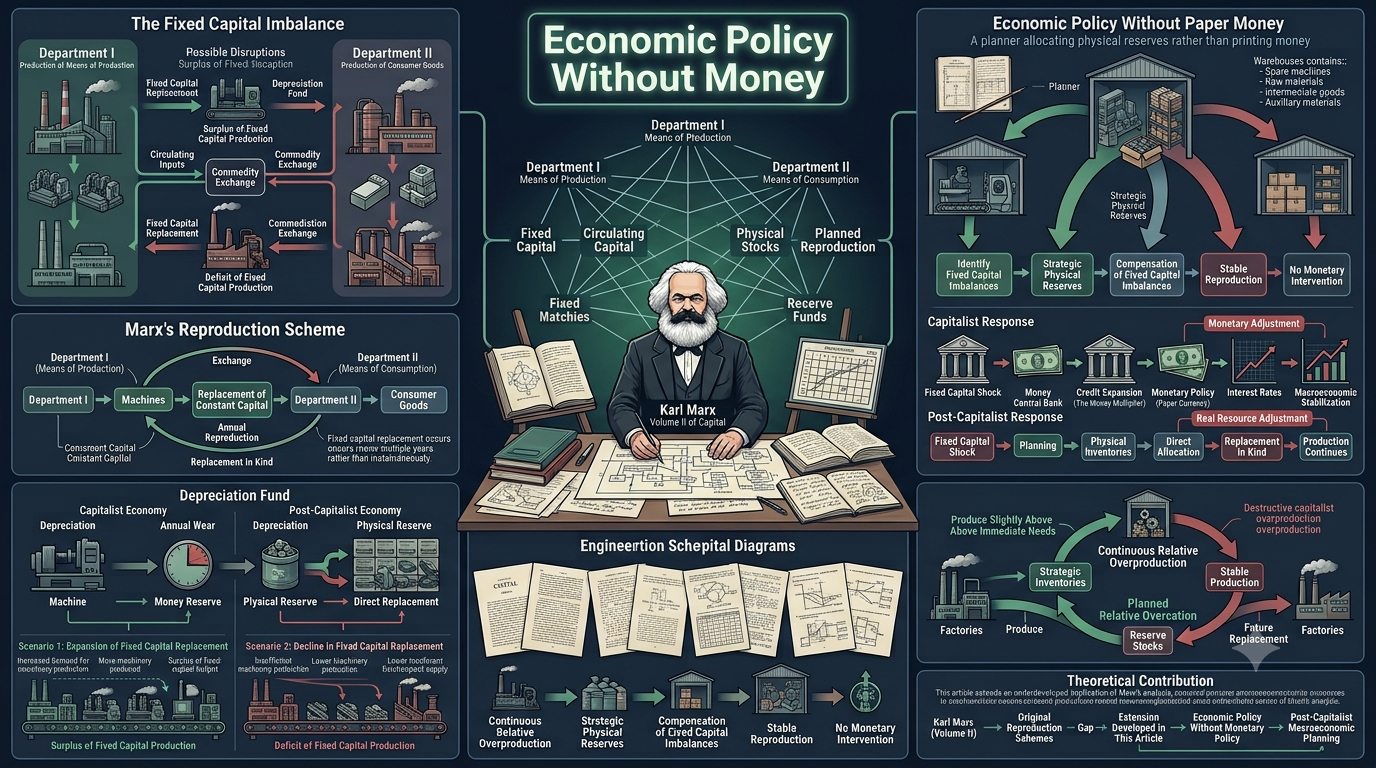
  • HOW TO CONDUCT ECONOMIC POLICY IN THE PRESENCE OF A FIXED CAPITAL SURPLUS OR DEFICIT WITHOUT RESORTING TO PAPER MONEY?

    HOW TO CONDUCT ECONOMIC POLICY IN THE PRESENCE OF A FIXED CAPITAL SURPLUS OR DEFICIT WITHOUT RESORTING TO PAPER MONEY?

    Can We Manage Fixed Capital Surpluses Without Money? — A Marxian Thought Experiment
    A Blog for the Curious Economist — and Everyone Else
    The Capital Question
    Marxian Political Economy Economic Policy 8 min read

    Can We Manage Fixed Capital Surpluses Without Money?

    An economist revisits a passage Marx left half-finished and asks: what if a post-capitalist society had to balance its machines, factories, and tools—without printing a single banknote?

    MG
    Based on the work of José Mauricio Gómez Julián
    Originally published • Revista Académica Contribuciones a la Economía • January 2016

    Most of us think of money as the universal lubricant of an economy—the thing that lets a shoe factory buy steel, and the steel mill pay its workers. But what happens when an economy decides it no longer needs money? Can it still keep its machines, buildings, and equipment in balance? That is the question José Mauricio Gómez Julián tackles in a compact, ambitious paper that draws directly on Karl Marx’s Capital, Volume II.

    Why Fixed Capital Matters

    Before diving in, let’s clarify what “fixed capital” means. In economics—especially in the Marxian tradition—a factory’s resources are split into two broad categories. Circulating capital is the stuff that gets used up quickly in production: raw materials, intermediate goods, energy. Fixed capital is the durable stuff—machinery, buildings, infrastructure—that transfers its value to the product gradually, over many production cycles, through wear and tear (what economists call “depreciation”).

    In any economy, these two types of capital need to exist in the right proportion. Too much fixed capital relative to circulating capital, and the machines sit idle for lack of materials. Too little, and the raw materials pile up with nothing to process them. Getting this ratio wrong creates either a surplus (overproduction of fixed capital) or a deficit (underproduction of fixed capital).

    The core insight is deceptively simple: even without money, an economy still needs a mechanism to absorb the shocks that come from uneven wear on its machines.

    The Two Scenarios: Surplus and Deficit

    Gómez Julián works through two thought experiments, both grounded in Marx’s two-sector model of reproduction (Sector I produces means of production—factories, machines; Sector II produces consumer goods). The logic is dense, but the intuition is elegant.

    1

    Scenario One

    Suppose the fixed capital used by the consumer-goods sector (Sector II) depreciates faster than expected in a given year. More machines need replacing now. Sector I sends more fixed-capital goods to Sector II, but its overall output for Sector II remains the same. The result: Sector I now produces more fixed capital than Sector II can absorb, while simultaneously Sector II needs less circulating capital (raw materials) because it is replacing machines rather than running them.

    Outcome → SURPLUS in fixed capital production
    2

    Scenario Two

    Now imagine the opposite: a smaller portion of Sector II’s fixed capital needs to be physically replaced this year (because less has worn out completely). That means less demand for new fixed-capital goods from Sector I. Meanwhile, the circulating capital flows remain unchanged. Sector I simply produces fewer fixed-capital items.

    Outcome → DEFICIT in fixed capital production

    In a capitalist economy, these imbalances ripple outward. The surplus scenario pushes more money into Sector I (as depreciation funds accumulate), but the actual exchange of goods shrinks. Money becomes a one-sided “means of purchase” rather than a smooth intermediary. In the deficit scenario, production contracts. Both situations, if left unmanaged, can trigger commercial crises—and in capitalism, those crises are cyclical, not one-off events.

    The Money Question

    Here is where the paper gets provocative. In a capitalist system, managing these imbalances requires monetary policy—central banks adjusting interest rates, governments running deficits, currencies being devalued. The entire toolkit of modern macroeconomics is, in one way or another, about using money to smooth out the frictions between production and exchange.

    But Gómez Julián asks: what if you remove money from the equation entirely? What if a post-capitalist society—one that has moved beyond the commodity form—tries to manage fixed capital imbalances without any monetary instrument at all?

    His answer is a policy of continuous relative overproduction: produce slightly more fixed capital and slightly more circulating capital than strictly necessary, and accumulate the excess as a strategic reserve.

    The logic works like this. If fixed capital wears out unevenly from year to year (sometimes more, sometimes less), a well-organized post-capitalist economy could buffer those fluctuations by maintaining reserve stocks of both fixed-capital goods and circulating-capital goods. When a year of heavy depreciation hits, the reserve steps in. When a year of light depreciation comes, the reserve grows. The goal is not maximum efficiency at every moment, but stability over time—a kind of industrial shock absorber.

    Why This Is Harder Than It Sounds

    The author is careful to note that this approach would be catastrophic in a capitalist economy. Continuous relative overproduction, without the discipline of a planned system, would generate commercial crises—overproduction in capitalism is not a “reserve strategy” but a trigger for collapse. The same policy looks entirely different depending on whether production is coordinated through market exchange or through conscious social planning.

    This is the key theoretical distinction: in a planned economy, overproduction is relative (producing more than immediate need, but deliberately) and continuous (a permanent buffer). In capitalism, overproduction is absolute (goods that cannot find buyers) and cyclical (recurring crises). Same material fact, radically different systemic consequences.

    A Critique the Author Couldn’t Ignore

    The paper ends with a sharp jab at Soviet Marxist economics. Gómez Julián points out that the standard Soviet reference text—the Dictionary of Marxist Political Economy by Borisov, Zhamin, and Makárova (1965)—never develops, or even mentions, this particular theoretical problem. The analysis is absent from the entries on “Fixed Capital,” “Simple Reproduction,” and “Extended Reproduction.” Marx himself only sketched it in embryonic form (Volume II, pp. 414–417), yet the author argues it is a “vital” issue for any theory of post-capitalist construction.

    His verdict on Soviet scholarship is unsparing: the Soviet economists, he suggests, never truly understood many of the theoretical foundations they claimed to be building on—a failure that history confirmed on November 9, 1989.

    • • •

    Why This Paper Deserves Your Attention

    You do not have to be a Marxist to find this paper interesting. At its heart, it is about a problem that any complex economy faces: how do you keep the right balance between durable infrastructure and the materials that flow through it? Modern economies answer this with monetary policy, fiscal stimulus, and market signals. Gómez Julián asks whether a fundamentally different kind of society could answer it with strategic reserves and conscious planning instead.

    Whether or not you find his vision persuasive, the thought experiment sharpens something important: our reliance on money as an economic management tool is not a law of nature—it is a feature of a particular system. And understanding why that system needs money is the first step toward imagining alternatives, or toward improving what we already have.

    This post is a summary and interpretation of the original research article. For the full theoretical development, including Marx’s formal apparatus, readers are encouraged to consult the paper directly: Gómez Julián, J. M. (2016), “¿Cómo Realizar Política Económica ante Superávit o Déficit de Capital Fijo sin Recurrir al Papel Moneda?”, Contribuciones a la Economía, ISSN 1696-8360.
    Original Article Gómez Julián, José Mauricio. “¿Cómo Realizar Política Económica ante Superávit o Déficit de Capital Fijo sin Recurrir al Papel Moneda?” Contribuciones a la Economía, January 2016, ISSN 1696-8360.
    Read the full paper here: https://dialnet.unirioja.es/servlet/articulo?codigo=9041512

    The Capital Question — Explaining the economics that shape our world, one paper at a time.

  • THE INFLUENCE OF JAMES MILL ON MODERN ECONOMIC SCIENCE

    THE INFLUENCE OF JAMES MILL ON MODERN ECONOMIC SCIENCE

    The Forgotten Father — James Mill and the Foundations of Modern Economics
    History of Economic Thought

    The Forgotten Father

    How James Mill quietly built the foundations of modern economics — and why nobody remembers

    Based on the research of José Mauricio Gómez Julián · Read the original article

    Picture the pantheon of classical economics. Adam Smith sits at the centre, David Ricardo stands nearby, Jean-Baptiste Say holds a modest plaque. Somewhere in the back, if he appears at all, you will find James Mill (1773–1836) — Scottish philosopher, historian, journalist, and the man the economist José Mauricio Gómez Julián argues we have been unjustly forgetting for nearly two centuries. In a concise but provocative article published in Economía & Región, Gómez Julián builds a meticulous case: Mill was not merely Ricardo’s friend and editor. He was, in several crucial respects, the intellectual architect behind ideas we now attribute to others — and the quiet originator of concepts that still animate central bank boardrooms today.

    What follows is a guided walk through that argument. No equations, no jargon — just the story of a mind that anticipated, with striking clarity, debates we are still having in the twenty-first century.

    I. The Law That Was Never Say’s

    If you have taken even a single semester of macroeconomics, you have encountered Say’s Law — the proposition that “supply creates its own demand.” It is one of the most cited principles in the history of the discipline, and it is routinely attributed to the French economist Jean-Baptiste Say.

    Gómez Julián’s article asks a simple, uncomfortable question: did Say actually come up with it first?

    The evidence points elsewhere. In 1807, an English writer named William Spencer published an argument containing the essential logic: that the annual produce of a country “always creates a market to itself,” and that when commodities seem to exceed demand, the real problem is merely a misallocation of productive effort among sectors, not a general glut. James Mill seized on this reasoning in his 1808 work Commerce Defended, presenting it with considerably more force and theoretical precision.

    “How great soever annual produce may be it always creates a market to itself; and that how great soever that portion of the annual produce which is destined to administer reproduction… its effects always are to render the country richer, and its inhabitants more opulent, but never to confuse or to overload the national market.” William Spencer (1807), cited by James Mill in Commerce Defended (1808)

    Three years later, in his 1821 Elements of Political Economy — the book Gómez Julián calls Mill’s “magnus opus” — Mill refined the idea further, embedding it in a broader theory of how supply, demand, and production costs interact over time. His formulation is careful and layered: relative prices are determined in the first instance by supply and demand, but ultimately by cost of production, because competition relentlessly pushes markets toward equilibrium.

    The article’s charge is direct: Say popularised an idea that was already circulating in English-language economics, and the discipline’s later canonisation of “Say’s Law” obscured its true origin. Gómez Julián does not mince words — he uses the term “plagiarism” (or rather, the article calls it “the least known plagiarism of the Classical Economists”).

    Whether one accepts that strong characterisation or prefers a milder framing of “parallel development,” the underlying historical point stands: Mill was articulating this foundational principle at least as early as Say, and arguably with greater analytical sophistication.

    II. Money, Prices, and the Seeds of Central Banking

    Here is where Mill’s contribution moves from historical curiosity to genuine intellectual substance. Gómez Julián argues that Mill was one of the finest exponents of the Quantity Theory of Money in his era — and, crucially, that he did so without falling into the contradictions that plagued later economists.

    The Quantity Theory, in its simplest form, says that the total amount of money in circulation determines the general level of prices. Mill stated it with remarkable directness:

    “It is not difficult to perceive, that it is the total quantity of the money in any country, which determines what portion of that quantity shall exchange for a certain portion of the goods or commodities of that country.” James Mill, Elements of Political Economy (1821)

    But the real surprise, for anyone accustomed to thinking of classical economists as rigid free-market purists, is what Mill argued next. He described two distinct circumstances under which a government might create money: first, by allowing it to “float freely” in the channels of circulation (essentially, an open mint where citizens bring bullion to be coined); and second, when the government wishes to control the quantity of money at its discretion.

    This is a startlingly modern framing. Unlike his friend David Ricardo, who frequently questioned any form of government monetary intervention, Mill was willing — even eager — to theorise about deliberate monetary management. He proposed that if the government wanted less money in circulation, it should raise the metallic value of the coinage (making each coin worth more); if it wanted more, it should lower it. The mechanism differs from modern interest-rate policy, of course, but the underlying logic — that a central authority should actively calibrate the money supply to achieve macroeconomic goals — is recognisably the ancestor of what every central bank does today.

    Why this matters

    The standard history of monetary policy tends to jump from the Currency School vs. Banking School debates of the 1840s straight to the Federal Reserve’s founding in 1913. Mill’s writing suggests that the intellectual groundwork for active monetary management was already being laid two decades earlier — and by a figure typically remembered, if at all, as a mere populariser of Ricardo.

    III. Trade Without Illusions

    Ricardo’s theory of comparative advantage is one of the most celebrated ideas in all of economics. Gómez Julián notes, however, that James Mill saw international trade through a rather different and more pragmatic lens.

    For Mill, the relationship between nations was essentially the same as the relationship between individual merchants: buy in the cheapest market, sell in the most expensive. He did not need the elaborate logical apparatus of comparative advantage to explain why trade was beneficial. The article suggests that Ricardo’s theory, far from being the inevitable culmination of classical trade thinking, was in some sense a detour — and that Mill’s simpler framework was closer to how commerce actually works.

    Moreover, Mill was one of the first economists to recognise that currency devaluation could be used as a tool for international competitiveness. The idea that a nation might deliberately weaken its exchange rate to boost exports is a staple of modern policy debates; Gómez Julián traces the logic back to Mill’s Elements.

    IV. Productive Labour, Unproductive Labour, and the Nature of Capital

    Adam Smith famously distinguished between “productive” and “unproductive” labour — a tailor makes something tangible, a servant does not. But Gómez Julián argues that Mill was the first economist to define these categories with genuine clarity, going beyond Smith’s somewhat impressionistic treatment.

    Mill also drew a related distinction between productive consumption and unproductive consumption — the idea that some spending builds future capacity while other spending merely satisfies immediate desires. Karl Marx, who read Mill carefully, admired the precision with which Mill laid out these ideas. In his 1844 Comments on James Mill, Marx praised the exposition with what he called Mill’s “customary cynical acumen and clarity.” It is an extraordinary compliment from a thinker not known for flattery.

    On the question of capital, Mill made further contributions that have been overlooked. He was among the first — alongside the lesser-known Samuel Bailey — to discuss capital accumulation in depth: specifically, what happens to industrial capital’s effects when the total amount of capital remains constant. Gómez Julián notes, fairly, that Mill made an error here (treating the portion of capital invested in labour-power as fixed), but the discussion itself was pioneering.

    Mill also drew a sharp conceptual line between the circulation medium used as capital (money deployed for productive investment) and the circulation medium used as a simple medium of exchange (money used for everyday purchases). Marx would later build extensively on this distinction in his own economic writings.

    V. Population, Egoism, and the Architecture of Political Economy

    Thomas Malthus is remembered for his theory that population tends to outstrip the food supply. Mill offered a strikingly different perspective: population density is ultimately determined by the needs of capital, not by any abstract biological tendency toward over-reproduction. In a single sentence, Mill redirected the population question from biology to political economy — a reorientation with implications that echo through later Marxist and institutional economics.

    “There is a certain density of population which is convenient, both for social intercourse, and for that combination of powers by which the produce of labour is increased.” James Mill, Elements of Political Economy (1821)

    On the question of self-interest, Gómez Julián argues that Mill’s treatment of egoism, private property, and production was clearer and deeper than Adam Smith’s in The Theory of Moral Sentiments. Marx summarised Mill’s position in a single lapidary phrase: “The limit of his need constitutes the limit of his production.”

    And then there is the matter of Mill’s intellectual architecture. His Elements of Political Economy is organised into four books:

    1. Production — how wealth is created.
    2. Distribution — how wealth is divided among social classes.
    3. Exchange — how commodities trade for one another, and the role of money.
    4. Consumption — how wealth is used, and under what conditions it expands or contracts.

    This four-part structure, elegantly simple, became the template for generations of economics textbooks. John Stuart Mill’s own celebrated Principles of Political Economy (1848) follows essentially the same outline — not a coincidence, given that James was his father and tutor.

    VI. The Teacher’s Shadow

    The final dimension of Mill’s influence is indirect but enormous. John Maynard Keynes, in The General Theory of Employment, Interest and Money, wrote that “‘classical economists’ was a name invented by Marx to refer to Ricardo, James Mill, and their predecessors — that is, to the founders of the theory that culminated with Ricardo.” Notice: Keynes lists James Mill first, before Ricardo.

    Beyond his own published work, Mill shaped the discipline through personal influence. He was David Ricardo’s closest intellectual confidant, his editorial advisor, and — as Gómez Julián emphasises — one of the principal mentors who encouraged Ricardo to write his masterwork. Sraffa’s monumental edition of Ricardo’s Works and Correspondence documents the extent of this influence, and Donald Winch’s Selected Economic Writings further confirms it.

    And of course, there is John Stuart Mill, arguably the most influential economist of the mid-nineteenth century, who received his entire early education from his father. Karl Marx, commenting acidly on the younger Mill’s monetary theories, observed that John Stuart had “his customary eclectic logic to embrace his father’s soup and at the same time the opposite” — a backhanded compliment to both Mills that inadvertently testifies to how deeply James Mill’s ideas had penetrated the discipline.

    The central claim

    Gómez Julián’s article does not argue that James Mill was a greater mind than Smith or Ricardo. It argues something subtler and, in its way, more important: that Mill was the connective tissue of classical economics — the thinker who synthesised scattered insights into coherent frameworks, who mentored the people we remember, and who anticipated policy ideas (monetary management, exchange-rate competitiveness) that would not become mainstream for another century. He was, in Keynes’s telling, a founder. And yet most economics programmes today never mention his name.

    · · ·

    A Final Thought

    History is written by the remembered. In economics, as in most fields, the canon narrows with each generation: a handful of names survive, and the rest fade into footnotes. Gómez Julián’s article is a reminder that those footnotes sometimes conceal ideas of startling originality and enduring relevance.

    James Mill may never have the name recognition of Adam Smith or John Maynard Keynes. But the next time you hear a central banker discuss money supply management, or a trade minister talk about exchange-rate strategy, or an economist invoke the idea that supply and demand are two sides of the same coin — spare a thought for the Scottish philosopher who got there first, and whose influence is still hiding in plain sight.

    — End —

  • Inflation Is (Not) Always And Everywhere A Monetary Phenomenon

    Inflation Is (Not) Always And Everywhere A Monetary Phenomenon

    Beyond the Phillips Curve — A Marxist Reinterpretation of Inflation
    Political Economy July 2025 · 8 min read

    Beyond the Phillips Curve

    A new study argues that inflation isn’t just about too much money chasing too few goods — it’s about how the capitalist class converts technological advantage into permanent profit.

    Most of us were taught a tidy story: when unemployment falls, inflation rises, and vice versa. This trade-off — called the Phillips Curve — has anchored central bank policy for decades. But what if that story is not just incomplete, but fundamentally misleading?

    A recent paper published in Realidad Económica by José Mauricio Gómez Julián argues exactly that. Using over fifty years of U.S. data (1968–2021), the study finds no significant long-run relationship between inflation and unemployment. Instead, it identifies a surprising positive link between technological change and inflation — and uses that finding to build a Marxist reinterpretation of what inflation actually does inside a capitalist economy.

    It’s a paper that challenges both mainstream economics and the popular imagination. Let me walk you through it.

    The Phillips Curve: A Love Story with Complications

    In 1958, New Zealand economist A.W. Phillips noticed an elegant regularity in British data: wages tended to rise faster when unemployment was low. Later economists generalized this into a policy menu: want less unemployment? Accept a bit more inflation. Want to tame prices? Brace for a recession.

    This trade-off became gospel in the 1960s. Central bankers thought they could fine-tune the economy like a thermostat — dial inflation up or down by adjusting demand. But the 1970s shattered that confidence. The U.S. experienced stagflation: high inflation and high unemployment at the same time, something the Phillips Curve said shouldn’t happen.

    Since then, economists have debated whether the Phillips Curve is dead, dormant, or merely sleeping. Gómez Julián sides with a more radical verdict: the long-run Phillips Curve doesn’t just flatten — it was never there to begin with.

    What does “long run” mean here? Mainstream economists already accept that the long-run Phillips Curve is vertical (meaning no permanent trade-off). But Gómez Julián goes further: he finds that even in shorter cycles, the supposed inverse relationship is statistically fragile — easily dissolved once you account for other variables, especially technological change.

    The Data, the Tools, and What They Found

    The study uses three complementary statistical approaches — each chosen for a reason:

    Bayesian Correlations

    Unlike classical statistics, which gives you a yes-or-no answer (“significant at 5%”), Bayesian analysis lets you say something more nuanced: “Given the data, here is the probability that this relationship is positive, negative, or nonexistent.” Applied to U.S. inflation and unemployment, the Bayesian results show no consistent inverse relationship. The data simply doesn’t support the Phillips Curve story with any confidence.

    Granger Causality

    This is a standard econometric test that asks: does knowing today’s unemployment help you predict tomorrow’s inflation (or vice versa)? If the Phillips Curve were real, the answer should be yes. Gómez Julián finds that the answer is generally no. Unemployment does not Granger-cause inflation in the U.S. data. What does show predictive power? Research and development spending.

    Error Correction Models (ECM)

    These models examine whether variables that drift apart over time eventually pull back together — like two dancers who briefly separate but remain on the same floor. The ECM results confirm that inflation and unemployment do not share a stable long-run equilibrium. They are, statistically speaking, dancing to different music.

    · · ·

    The Surprising Link: Technology Drives Inflation

    Here is the paper’s most provocative finding: R&D expenditure and inflation move together positively. When firms invest more in technology, inflation tends to rise — not fall, as you might expect from a productivity-enhancement standpoint.

    Why would better technology lead to higher prices? To answer this, Gómez Julián turns to Marx — specifically, to the distinction between two types of surplus value.

    Capitalist innovates
    (new machinery, process)
    Extraordinary surplus value
    (temporary advantage)
    Rivals adopt technology
    Inflation absorbs the gap
    Relative surplus value
    (permanent for the class)
    Fig. 1 — The mechanism proposed by Gómez Julián, simplified.

    Two Kinds of Surplus Value: A Quick Primer

    If you’re not steeped in Marxist theory, don’t worry — the distinction is intuitive.

    Absolute surplus value is what a capitalist gets by making workers work longer or harder for the same pay. It’s the old-fashioned squeeze. Relative surplus value, by contrast, comes from making production cheaper — through technology, efficiency, better organization — so that the value of labor-power (i.e., the cost of maintaining a worker) falls, even if wages don’t.

    Now imagine a single firm introduces a breakthrough technology. It can produce goods faster and cheaper than its competitors. For a while, it earns extraordinary surplus value — a premium profit that exists only because it’s ahead of the pack. But here’s the catch: once competitors adopt the same technology, that advantage vanishes. The extraordinary surplus value disappears.

    Gómez Julián’s argument is that inflation is the mechanism through which this temporary advantage gets converted into a permanent one. How? As the innovating firm’s higher productivity drives down unit costs, prices don’t fall proportionally — instead, the general price level adjusts upward. The gap between the old cost structure and the new one gets absorbed by inflation. What was a one-time windfall for the innovator becomes a structural shift in profitability for the entire capitalist class.

    Inflation, in this reading, is not a policy error or a monetary accident. It is a functional mechanism of capitalist accumulation — one that converts technological advantage into lasting class-wide profit.

    What This Means for Policy

    If the paper is right, the implications are significant:

    For central bankers: If inflation isn’t primarily a monetary phenomenon — if it’s rooted in the structural dynamics of production and profit — then raising interest rates to fight inflation is treating the symptom, not the disease. You might cool the economy, but you’re not addressing the engine that generates inflation in the first place.

    For mainstream economists: The Phillips Curve may be less a stable empirical law and more a historical coincidence — a relationship that appeared to hold in a particular postwar context and has been propped up by theoretical convenience ever since. The paper adds to a growing body of evidence that the curve has become unreliable as a guide to policy.

    For non-economists: This paper reframes inflation as a political question, not just a technical one. If inflation systematically benefits capital at the expense of labor — by preserving the gains of innovation for the capitalist class while workers’ purchasing power erodes — then debates about inflation are, at their core, debates about distribution and power.

    A note of caution The paper uses R&D spending as a proxy for technological change. This is standard in the literature, but it’s not a direct measure of innovation. R&D spending can reflect many things — tax incentives, defense contracts, speculative bubbles in tech. The correlation Gómez Julián finds is suggestive and theoretically grounded, but it warrants further investigation with additional proxies and across different economies.
    · · ·

    A Challenge to Orthodoxy

    What makes this paper worth reading — whether you agree with it or not — is that it does something many economists avoid: it takes a heterodox theoretical framework seriously and tests it empirically. This isn’t armchair Marxism. It’s Bayesian statistics, Granger causality, and error correction models applied to five decades of data. The methodology is conventional; the interpretation is not.

    The mainstream view treats inflation as essentially a monetary phenomenon — too much money, not enough stuff. Milton Friedman’s famous dictum that “inflation is always and everywhere a monetary phenomenon” still echoes through central banks worldwide. Gómez Julián doesn’t deny that money supply matters. But he argues it’s not the whole story — and may not even be the most important part.

    In his framework, the relationship between technology, surplus value, and prices is structural. It doesn’t depend on whether a central bank is dovish or hawkish. It’s embedded in the logic of capitalist production itself.

    So, Is the Phillips Curve Dead?

    Probably not entirely. There are short-run contexts where demand pressures do push prices up, and the Phillips Curve captures something real about those moments. But the paper pushes us to ask harder questions: What determines the baseline around which those fluctuations occur? Why has inflation behaved the way it has over half a century, regardless of the unemployment rate?

    Gómez Julián offers a provocative answer: inflation is the economy’s way of metabolizing technological progress into profit. It’s not a bug in the system. It’s a feature.

    Whether you find that convincing depends, in part, on your theoretical priors. But the data doesn’t lie about what it doesn’t show: a reliable Phillips Curve. And that, at minimum, should give everyone — mainstream, heterodox, and curious layperson alike — something to think about.