
Espartaco

“Is that to say we are against Free Trade? No, we are for Free Trade, because by Free Trade all economical laws, with their most astounding contradictions, will act upon a larger scale, upon the territory of the whole earth; and because from the uniting of all these contradictions in a single group, where they will stand face to face, will result the struggle which will itself eventuate in the emancipation of the proletariat.”

Karl Heinrich Marx · Marx-Engels Collected Works, Vol. VI, p. 290

EnglishEspañol

Tag: leave-future-out cross-validation

  • EconCausal: An R Package That Takes Causal Inference in Time Series Seriously

    EconCausal: An R Package That Takes Causal Inference in Time Series Seriously

    You can also find this library at CRAN and download it directly from R and RStudio.

    You found a relationship in your data. It’s statistically significant. The coefficients are clean. But here’s the question that keeps rigorous researchers up at night: will this relationship still hold six months from now?

    That question — whether a relationship between economic variables is real and durable, not just a fluke of the particular sample you happened to look at — is exactly what the EconCausal R package was built to answer.


    What Problem Does EconCausal Solve?

    Causal inference in time series data is notoriously tricky. Standard regression can tell you that two variables move together. It cannot tell you why, or whether that co-movement will persist when the economic regime shifts — which it inevitably will.

    EconCausal addresses this challenge by combining three well-established econometric methodologies into a single, reproducible pipeline. What makes it distinctive is not any single technique — each component has solid academic pedigree — but rather the orchestration: a standardized protocol that forces every candidate relationship through rigorous pre-testing, proper temporal validation, and explicit decision rules before declaring a finding.

    Think of it as a quality-control assembly line for causal claims in time series.


    The Three Approaches

    EconCausal implements three methodological frameworks, each capturing a different aspect of what “causality” can mean in temporal data. Using all three gives you complementary perspectives rather than relying on a single method’s assumptions.

    1. Error Correction Models with MARS (ECM-MARS)

    The idea: Many economic variables share a long-run equilibrium relationship but deviate from it in the short run. An Error Correction Model (ECM) captures both dimensions — the long-run cointegrating relationship and the short-run adjustment dynamics.

    EconCausal enhances the classical ECM by replacing its usual linear regression engine with Multivariate Adaptive Regression Splines (MARS), a flexible non-parametric method developed by Jerome Friedman in the early 1990s. This matters because real-world adjustment mechanisms are often nonlinear: variables may correct slowly when deviations are small but snap back aggressively when deviations cross certain thresholds. MARS can detect these threshold effects automatically without you having to specify them in advance.

    What the protocol does in practice:

    • Tests whether the variables are integrated of order one (I(1)) — a prerequisite for cointegration analysis
    • Runs both the Engle-Granger and Johansen cointegration tests, applying an “either” rule: if either test finds evidence of cointegration, the analysis proceeds
    • Controls for serial correlation and heteroskedasticity using HAC-consistent standard errors
    • Fits the ECM with MARS as the regression engine
    • Validates the relationship using rolling-origin cross-validation
    • Evaluates the model using a dual criterion (more on this below)

    Why two cointegration tests? Because Engle-Granger and Johansen have complementary strengths. Engle-Granger is intuitive and straightforward but can miss cointegrating relationships in multivariate settings. Johansen’s approach is more powerful in higher dimensions but relies on stricter distributional assumptions. Requiring only one of them to flag significance is a pragmatic compromise that reduces false negatives without being reckless about false positives.

    2. Bayesian Structural Time Series (BSTS)

    The idea: Decompose a time series into interpretable structural components — trend, seasonality, regression effects — and do so within a fully Bayesian framework that quantifies uncertainty at every level.

    BSTS, originally popularized by Google’s CausalImpact package and the work of Scott and Varian (2014), models the data-generating process as a state-space system. The key innovation in EconCausal’s implementation is the use of spike-and-slab priors for automatic variable selection. This is a Bayesian regularization technique that effectively asks: “Which candidate predictors actually belong in this model?” — and it does so probabilistically, rather than relying on stepwise procedures or arbitrary p-value cutoffs.

    What makes it useful for causal inference:

    • The structural components absorb confounding patterns (trends, seasonality) that might otherwise masquerade as causal relationships
    • Spike-and-slab priors guard against overfitting by aggressively shrinking irrelevant predictors toward zero
    • The Bayesian framework produces probabilistic forecasts — not just point predictions, but full posterior distributions — which naturally give you calibrated prediction intervals
    • It handles the “what would have happened without the intervention” question, which is central to impact evaluation

    3. Bayesian GLM with AR(1) Errors (BGLM-AR1)

    The idea: Fit a Bayesian generalized linear model but explicitly account for temporal dependence in the residuals through a first-order autoregressive error structure.

    This might sound like a niche technical detail, but it addresses one of the most common mistakes in applied econometrics: ignoring autocorrelation in regression residuals. When residuals are correlated over time, standard errors are wrong, confidence intervals are too narrow, and you end up being more confident in your results than you should be.

    By modeling the residual autocorrelation directly with an AR(1) structure and using Hamiltonian Monte Carlo (HMC) sampling via Stan, the BGLM-AR1 approach produces valid inference even when the data have strong temporal dependence. The priors are weakly informative and calibrated for standardized variables, which means they provide regularization without dominating the data.

    The dual evaluation criterion: This is where EconCausal’s protocol really distinguishes itself. A relationship is only accepted if it improves both:

    1. Predictive density (measured by Expected Log Predictive Density, or ELPD, estimated via Pareto-Smoothed Importance Sampling Leave-One-Out cross-validation — PSIS-LOO)
    2. Point forecast accuracy (measured by RMSE)

    Requiring improvement on both dimensions simultaneously is stricter than most practitioners apply. A model might improve point forecasts while worsening the calibration of its uncertainty estimates, or vice versa. EconCausal demands both.


    What Makes EconCausal Different: The Protocol

    You might be thinking: “Most of these individual techniques already exist in other R packages — brms and Stan for Bayesian modeling, the ecm package for error correction models, bsts and CausalImpact for structural time series.” And you’d be right.

    The novelty of EconCausal is not in inventing new statistical methods. It lies in integrating them into a single, standardized protocol with explicit decision rules, thresholds, and validation procedures that run automatically.

    Here’s what that means concretely:

    Temporal Stability Validation

    Rather than evaluating a model on a single train-test split, EconCausal uses Leave-Future-Out (LFO) cross-validation with configurable windows and horizons. The system repeatedly:

    1. Trains on data up to a cutoff point
    2. Forecasts into the future
    3. Evaluates forecast accuracy
    4. Slides the cutoff forward
    5. Repeats

    A relationship is only declared “stable” if it performs consistently across multiple temporal folds — not just one lucky window. The package reports a support metric: the proportion of temporal folds where the relationship holds up.

    Dual Decision Rules with Explicit Thresholds

    Every candidate relationship must clear both the Bayesian bar (ELPD improvement) and the frequentist bar (RMSE reduction). These are not vague guidelines — the protocol applies explicit numerical thresholds and includes tie-breaking rules for ambiguous cases.

    A Single Reproducible Pipeline

    From data loading through pre-testing, model fitting, temporal validation, and final go/no-go decisions — everything runs in one pipeline. This eliminates the researcher degrees of freedom that plague so many applied studies, where hundreds of analytical choices are made invisibly along the way.

    An independent novelty assessment included in the package’s documentation compared this protocol against both the academic literature and existing software frameworks. The finding: while all the building blocks are state-of-the-art and well-documented in the literature, no existing academic paper or software package was found that implements the same end-to-end protocol with the same combination of pre-tests, dual decision rules, support thresholds, and temporal validation.

    ApproachComponents = State of the Art?Identical Protocol in Literature?Identical Protocol in Existing Software?
    BGLM-AR(1)YesNoNo
    ECM-MARSYesNoNo (though ecm + earth approximates the model-fitting step)
    BSTSYesNoNo

    Who Should Use EconCausal?

    The package was originally designed for economic research — specifically, examining production-circulation relationships — but its applicability extends to any domain where you need to answer questions like:

    • Does X cause Y, or is it the other way around? The temporal structure of the methods naturally distinguishes between “X leads Y” and “Y leads X.”
    • Is this relationship robust across time? The rolling-origin validation directly tests temporal stability.
    • Are there nonlinear dynamics at play? The MARS component in ECM-MARS can detect threshold effects and nonlinear adjustment speeds.
    • How certain can we be? The Bayesian components (BSTS and BGLM-AR1) provide full uncertainty quantification, not just point estimates.

    This makes it useful for:

    • Academic researchers conducting empirical macroeconomics, financial economics, or applied econometrics
    • Policy analysts evaluating whether proposed policy relationships will hold across different economic conditions
    • Data scientists in finance who need to move beyond correlation to directionality and stability
    • Graduate students learning causal inference methods who want a pedagogical tool that enforces methodological discipline

    Getting Started

    Installation is straightforward:

    # Install from GitHub
    remotes::install_github("IsadoreNabi/EconCausal")
    # On Windows, if vignette building fails:
    remotes::install_github("IsadoreNabi/EconCausal", build_vignettes = FALSE)

    The package depends on a modern Bayesian computing stack — cmdstanr for Hamiltonian Monte Carlo sampling, loo for PSIS-LOO computation, and bsts for structural time series components — so make sure your R environment is up to date.


    A Note on What EconCausal Is Not

    It’s worth being explicit about the boundaries:

    • It is not a magic wand. If your data are fundamentally unsuitable for causal inference (too few observations, structural breaks that dominate the signal, measurement error in the variables), EconCausal will not rescue you. Its value lies in applying rigorous methods correctly and transparently — not in overcoming the limitations of your data.
    • It does not replace domain knowledge. Statistical evidence for a stable, directional relationship is necessary but not sufficient for a causal claim. You still need a theoretical mechanism, an understanding of potential confounders, and judgment about the plausibility of the identifying assumptions.
    • It does not invent new mathematics. Its contribution is the protocol — the disciplined, reproducible integration of established techniques into a pipeline with explicit, auditable decision rules.

    The Bottom Line

    EconCausal occupies a valuable niche in the R ecosystem. While individual components of its methodology are available elsewhere — Bayesian GLMs in brms, BSTS in the bsts package, ECM in the ecm package — no other tool packages them into a single protocol that systematically tests temporal stability, applies dual evaluation criteria, and produces reproducible, auditable results.

    If your work involves making causal claims from time series data — and you care about whether those claims will survive contact with the future — EconCausal deserves a serious look.

    Repository: github.com/IsadoreNabi/EconCausal


    References for the underlying methodologies: Engle & Granger (1987), Johansen (1991), Friedman (1991), Scott & Varian (2014), Vehtari et al. (2017), Hyndman & Athanasopoulos (2021). See the package documentation for the complete bibliography.
  • When the Textbook Test Fails: How HTDV Brings Rigor to Dependent, Unbalanced Data

    When the Textbook Test Fails: How HTDV Brings Rigor to Dependent, Unbalanced Data

    You can also find this library at CRAN and download it directly from R and RStudio.

    The problem hiding in your data

    Picture a straightforward question: Is the average inflation rate in the United States meaningfully different from zero? You have monthly data going back decades. A classical t-test would seem like the natural tool — and it would be quietly, systematically wrong.

    The reason is that inflation figures do not bounce around independently. January’s number carries information about February’s. This autocorrelation corrupts the standard error that the t-test relies on, inflating the false-positive rate well beyond the nominal 5% you think you are signing up for. The same problem afflicts yield spreads, stock returns, sectoral profitability, regional employment — virtually any real-world time series you might want to compare.

    Now make it harder. The two groups you are comparing have different sample sizes — one sector has twenty years of data, another only five. The data may have heavy tails you cannot rule out. And your sample is finite, which means the asymptotic guarantees printed in your econometrics textbook are promises that may not have been kept yet.

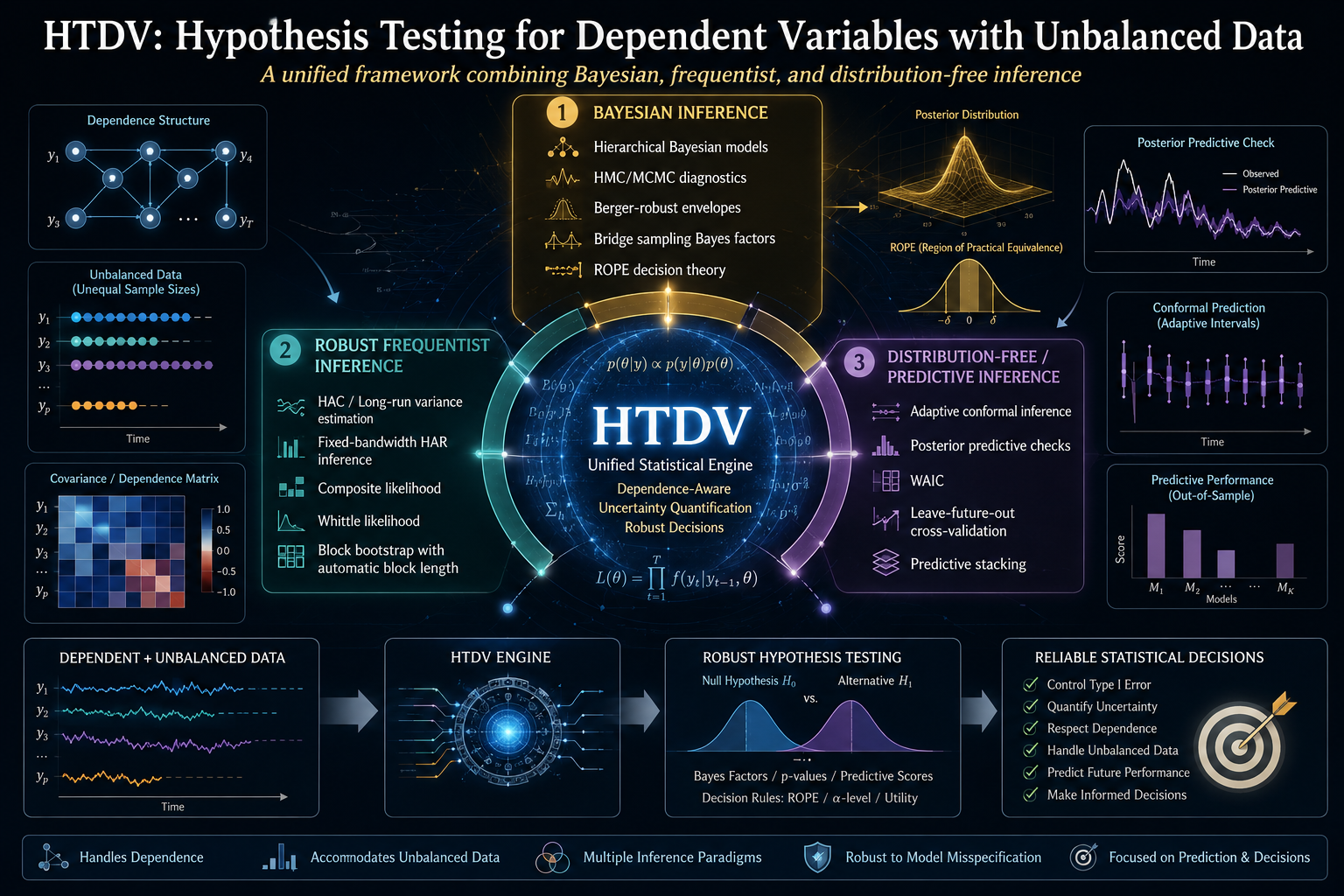
    This is the terrain HTDV was built for. Short for Hypothesis Testing for Dependent Variables with Unbalanced Data, HTDV is an R package that answers a deceptively simple question — do these dependent, possibly unequally-sized samples come from the same population? — under the worst combination of conditions an applied statistician is likely to encounter.

    The central idea: triangulation, not trust

    The most common approach to dependent data is to reach for a single robust method — a heteroskedasticity-and-autocorrelation-consistent (HAC) standard error, say, or a block bootstrap — and hope it is calibrated. HTDV takes a structurally different stance: run three independent inferential methods in parallel and expose the disagreement between them as a signal.

    The three layers are:

    1. A hierarchical Bayesian fit via Hamiltonian Monte Carlo (HMC), implemented in Stan. This layer builds a full probability model of the data-generating process, places weakly informative priors on the dependence parameters, and produces a posterior distribution for the quantity of interest.
    2. A fixed-bandwidth HAR Wald test in the frequentist tradition of Kiefer and Vogelsang (2005). Rather than letting the bandwidth grow with the sample in the usual way, it holds the bandwidth at a fixed fraction of the sample size. This produces a non-standard asymptotic distribution that is better calibrated in finite samples than the conventional chi-square approximation.
    3. A stationary block bootstrap (Politis and Romano, 1994) with automatic block-length selection (Patton, Politis, and White, 2009). This resamples the data in blocks long enough to preserve the dependence structure, then constructs confidence intervals from the resampled distribution.

    A fourth, distribution-free layer — adaptive conformal inference (Gibbs and Candès, 2021) — is available for online prediction settings where no parametric assumption is palatable.

    The logic is forensic. Where all three layers agree, your conclusion is robust. Where they disagree, the pattern of disagreement tells you something specific about your data. If the Bayesian interval is dramatically wider than the HAR or bootstrap interval, your series likely has strong temporal persistence, and the asymptotic critical values that HAR and bootstrap rely on are losing their reliability. That gap is not a bug — it is the most informative thing the framework can show you.

    Why a single method is not enough

    It is fair to ask: if the Bayesian layer is the most reliable, why not just use it and discard the others? The answer is that each layer has a regime where it is the appropriate tool, and the framework’s job is to make the regime visible.

    HAR inference is computationally cheap — sub-second on typical data — and well-calibrated when persistence is low to moderate and sample sizes are large enough for asymptotics to bite. The block bootstrap shares those advantages while making fewer distributional assumptions. The Bayesian layer is the most computationally expensive (each fit can take tens of seconds) but is the only one that maintains nominal calibration under strong persistence at finite sample sizes, because it models the dependence explicitly rather than relying on asymptotic corrections.

    The package ships with a pre-registered factorial Monte Carlo study — 1,024 cells crossing sample size, autocorrelation, tail heaviness, imbalance ratio, and location shift, with 500 replications per cell across all three inferential layers — and the results are unambiguous. The Bayesian layer holds nominal size (mean 0.056 against a target of 0.05) and nominal coverage (mean 0.944 against a target of 0.95) across the entire grid. HAR and bootstrap, by contrast, inflate dramatically in the worst corners: under strong persistence and small samples, HAR’s empirical rejection rate under the null reaches 0.60, and its coverage drops to 0.29.

    The narrowness of the HAR and bootstrap intervals in those corners is not a sign of precision. It is a sign of miscalibration — the intervals are confidently wrong.

    The theory that holds it together

    Running three different methods on the same data and comparing the answers is sound practice, but it raises a mathematical question: under what conditions are the three methods even addressing the same inferential target? A Bayesian posterior on a triangular-array likelihood and a HAR-Wald statistic on a mixingale process are, on their face, different objects.

    HTDV’s theoretical backbone is a metric equivalence theorem that resolves this concern. The framework identifies three structurally distinct ways real-world data can violate the independence assumption — each corresponding to a different law-of-large-numbers regime:

    • Triangular Arrays Convergence (TAC): information accumulates through hierarchical aggregation. Think of input-output tables disaggregated into ever-finer sectors, where each “row” of the array adds more observations.
    • Weighted Sums with Correlation (WSC): the observations share a cross-sectional covariance structure. Regional markets that move together, trade flows between linked economies.
    • Mixingale Process Convergence (MPC): temporal memory that decays smoothly over time. Forecast errors, model residuals, prediction intervals that gradually lose contact with the past.

    The theorem proves that, under α-mixing with polynomial decay rate γ > 1 and finite moment conditions, these three regimes induce strictly equivalent metrics on the space of hypothesis-testing problems. The equivalence comes with explicit, computable finite-sample constants — exposed by the function htdv_equivalence_constants() — that tell you the maximum slack when translating a conclusion from one regime to another. For typical parameter values (γ = 2, q = 6, n = 500), the conversion slack is about 18%, a margin that is usually irrelevant for a hypothesis-testing decision.

    This is what makes the three-layer architecture mathematically well-defined rather than merely pragmatic. Without the equivalence theorem, comparing a Bayesian result on a TAC dataset with a HAR result on a WSC dataset would be comparing apples and oranges. The theorem certifies that the metrics are coercible to one another with computable error.

    The dependence assumption, plainly

    The framework assumes that the data are α-mixing with polynomial decay — meaning that the statistical dependence between observations dies off as they get farther apart in time, and it does so fast enough (at a rate faster than 1/k) that the long-range correlations are summable. This is a mild condition satisfied by most stationary time series in econometrics and finance, including ARMA processes, GARCH models, and a broad class of Markov chains.

    It is not satisfied by long-memory processes (where dependence decays more slowly than 1/k) or by unit-root processes (where dependence does not decay at all). The framework is honest about these limitations: it will fit near-unit-root data, but the posterior will widen correspondingly — which is the correct answer. For explicit unit-root testing, the standard ADF or Phillips-Perron tools remain the right choice.

    The Bayesian engine

    The hierarchical Bayesian core fits Stan models via the No-U-Turn Sampler (NUTS), the state-of-the-art Hamiltonian Monte Carlo variant. The models are parameterized around an AR(1) structure — the mean θ, the autocorrelation φ, and the innovation scale σ — with hierarchical priors on the dependence nuisance parameters that are weakly informative enough to respect admissible ranges without overwhelming the data.

    Five likelihood backends are available, corresponding to the three convergence regimes plus two parametric likelihood families: the Whittle likelihood (which works in the frequency domain, comparing the observed periodogram to a theoretical spectral density) and the composite likelihood (which works in the time domain, combining conditional densities over short blocks). Both are well-established in the time-series literature; the choice between them depends on whether you have more confidence in your spectral model or your conditional density model.

    A distinctive feature is the Berger-robust envelope — a method for combining posteriors across multiple fitted models into a single, wider posterior that hedges against the worst-likelihood-specification scenario. If you are unsure whether the Whittle or composite likelihood better describes your data, the envelope gives you an inferential answer that is honest about that uncertainty rather than forcing an arbitrary choice.

    After sampling, every fit must pass a five-gate diagnostic check before its posterior is admissible: split-R̂ below 1.01, bulk and tail effective sample sizes above 400, zero post-warmup divergences, and energy Bayesian fraction of missing information (E-BFMI) above 0.3. These are the standard HMC convergence diagnostics from the Stan ecosystem, enforced as a gate rather than offered as a suggestion.

    The validation: visible in the data

    The most compelling aspect of HTDV is that it does not merely claim to be well-calibrated — it ships the evidence. Two validation datasets are bundled with the package.

    The first is the factorial simulation described above, with its 3,069-row summary table accessible as a package dataset. The headline finding — that the Bayesian layer is the only one maintaining nominal calibration across the full design — is not an assertion but a reproducible fact. The full study took 31 hours on a 16-core workstation; the scripts to regenerate it from scratch are shipped in the package repository.

    The second is a set of three external benchmarks against published references on public-source data:

    • Post-1984 US CPI inflation, compared against Stock and Watson (2007).
    • Shiller’s log-CAPE ratio, compared against Campbell and Shiller (1998).
    • The US–Canada 10-year yield differential, compared against the naive iid Welch baseline.

    All three layers reproduce all three references with agreement in every case. But the width of the agreement tells the real story. The interval widths scale monotonically with the persistence of the underlying series. At moderate persistence (φ ≈ 0.45, the inflation series), the Bayesian interval is actually narrower than HAR — 0.81 times its width. At high persistence (φ ≈ 0.97, the CAPE series), the Bayesian interval is 2.8 times wider. At near-unit-root persistence (φ ≈ 0.99, the yield differential), it is 15 times wider.

    This gradient is the framework’s central empirical finding. Both layers are technically asymptotically valid. Only the Bayesian layer accounts honestly for the finite-sample uncertainty inflation that occurs as φ approaches 1. The HAR and bootstrap intervals do not widen because they know more — they fail to widen because their asymptotic critical values have not yet caught up with the data.

    When to use it — and when not to

    HTDV is the right tool when your data are time-dependent or spatially dependent, when your samples are of unequal size, when you suspect heavy tails but cannot rule them out, and when you need an inferential answer (a test or an interval) rather than a prediction. It is particularly valuable when the stakes are high enough that you want your conclusion to survive methodological scrutiny — the framework ships its own validation evidence precisely so that a reviewer can interrogate the calibration claims rather than taking them on faith.

    It is the wrong tool when your data are genuinely independent with finite variance — classical methods are simpler, equivalent, and faster. It is also not designed for long-memory processes, explicit unit-root testing, structural breaks (unless you segment the sample first), or forecasting. The framework is built for hypothesis testing and parameter estimation under uncertainty, not for predictive accuracy.

    An open architecture

    The package exposes its full infrastructure: the simulation engine (htdv_simstudy()), the equivalence constants calculator, the diagnostic suite, the posterior-predictive checks on dependence statistics, and the decision tools — ROPE-based decisions (Kruschke, 2018), bridge-sampling Bayes factors, WAIC and leave-future-out cross-validation, and predictive stacking (Yao, Vehtari, Simpson, and Gelman, 2018). Every function is documented with its underlying reference, so the user can trace any method back to its source.

    The complete function reference, mathematical foundations, tutorial walkthroughs (oriented toward novices, applied statisticians, and mathematicians respectively), and the full validation narrative are in the HTDV Wiki on GitHub. The package is installed with a single command — remotes::install_github("IsadoreNabi/HTDV") — and requires rstan as its only hard dependency.

    The larger point

    HTDV embodies a methodological philosophy worth stating explicitly: when no single inferential method is universally valid in the finite-sample regime, the honest response is not to pick the best one and hide its limitations, but to run several and make the disagreement visible. The framework’s value is not that it always gives you a narrower interval or a more powerful test. Its value is that it shows you — concretely, quantitatively — where your inference is on solid ground and where it is standing on asymptotic ice.

    The validation evidence makes this concrete. In 98% of the simulation cells, the Bayesian layer alone passes the calibration benchmarks. The HAR and bootstrap layers pass in the regime where asymptotics have bitten — low persistence, large samples — and fail predictably outside it. The framework does not hide that failure. It turns it into a signal.

    That signal is the product.


    HTDV is released under the MIT license. The companion paper, full validation vignette, and reproducibility scripts are available at github.com/IsadoreNabi/HTDV. For the complete mathematical foundations, function reference, and tutorials, see the project wiki.