
Selecting Explanatory Variables in Statistical Models
Parsimony, structure, prediction, and methodological critique
Selecting a model requires deciding which relationships to preserve and how to test their consequences. This exposition connects philosophical discussion of parsimony with a reproducible comparison of 128 regressions for the fifty U.S. states. It presents selection criteria, derives PRESS, distinguishes influence from prediction error, and validates the entire procedure. Its central result—four predictors and an outer RMSE of 0.793 years under AIC selection—remains conditional on the model family, historical data, and analytical purpose.
1. Select for a specific question
A statistical model organizes relationships among observed quantities through assumptions about a population or process. Selecting explanatory variables means delimiting a representation: deciding which terms to retain, what information they contribute, and what uncertainty the decision introduces. The goal is more than shortening a list of columns. The scientific question, measurement quality, design structure, and intended use all matter.
Three tasks should be distinguished. Description summarizes associations within the data. Prediction approximates responses for observations that did not participate in fitting. Causal explanation identifies what would change under an intervention, requiring additional substantive and identification assumptions. An observational regression selected by AIC does not automatically answer that last question.
| Purpose | Central decision | Required evidence |
|---|---|---|
| Description | Summarize relationships clearly | Measurement, fit, and diagnostics |
| Prediction | Reduce out-of-sample loss | Validation of the entire procedure |
| Causality | Identify a defined effect | Design, temporal order, and confounding control |
The word explanatory, commonly used to denote a predictor, does not guarantee a mechanistic explanation. A predictive variable may proxy other conditions; a confounder may need to remain even when its coefficient fails a conventional threshold. Before automation, define the candidate universe and any variables that scientific reasoning requires retaining.
2. Parsimony, abstraction, and material structure
The principle of parsimony discourages unnecessary complications when several representations are adequate for a purpose. Its historical connection to Occam’s razor does not make simplicity a guarantee of truth or the exclusive property of one probabilistic school. Adequacy must be justified: a short description may omit a decisive relationship, while a long one may capture noise.
From the standpoint of Dialectical Materialism, scientific abstraction can be understood as a conceptual reconstruction of objective, historically determined relationships. Particular and general determinations are connected: concepts do not exist independently of all material activity, but their content is not merely an arbitrary collection of names. Within this framework, variable reduction should be assessed by the determinations it preserves and the mediations it removes. This is a philosophical interpretation of modelling, not a selection theorem.
The distinction between outward appearance and internal connection is central to Marx’s critique of representations of economic relations in Capital, volume III, chapter 48 (Marx, 1894/1999). Carefully applied to statistics, it encourages questions about why an association appears and under which conditions it recurs. It does not justify inferring a social cause from a coefficient’s sign or declaring the shortest model true.
The economy of a representation must remain subordinate to the adequacy of the relationships it represents.
Four meanings of complexity should be separated: the complexity of a material phenomenon, the parameter count of a representation, an algorithm’s execution cost, and the difficulty of interpreting its output. An efficient algorithm can search a large model family; a small parameter set can describe a complex process. Analogies across these levels are useful when their limits are explicit.
A rigorous critique of nominalism or subjectivism requires its own arguments. Associating Occam’s name with a penalty formula is insufficient, as is treating every prior distribution as an arbitrary choice. Practical objectivity is strengthened by explicit assumptions, tests of consequences, and sensitivity analysis in both frequentist and Bayesian procedures.
3. Linear models, assumptions, and hierarchy
Consider the conditional mean model y = Xβ + ε. The design matrix X has n rows and p columns; p includes the intercept. With full column rank and n > p, the ordinary least squares estimator and projection matrix are:
The formula describes the algebraic solution; unbiased estimation of β requires E(ε | X) = 0. The classical variance σ²(XᵀX)−1 requires Var(ε | X) = σ²I. Conditional normality gives exact t and F distributions for a specification fixed in advance. A selection algorithm does not establish these conditions. Numerical implementation should use QR, as lm() does, rather than explicitly forming an inverse.
Term hierarchy should be distinguished from multilevel models. In the former sense, a specification containing xz usually retains x and z; one containing x² usually retains x. This is a construction and interpretation rule, especially useful under changes of origin and scale. Substantive restrictions may justify exceptions. In the latter sense, hierarchy describes levels of variation, such as people within regions, often with random effects.
A fixed-degree polynomial regression remains parametric and linear in its coefficients even though its response curve is nonlinear in x. Centering can reduce some collinearity; orthogonal bases re-express the same fitted space when degree is held fixed. Orthogonal columns do not establish statistical independence of the original variables. Transformation constants must be retained for prediction, and unjustified extrapolation should be avoided (Kutner et al., 2005).
4. What each criterion measures
RSS denotes the residual sum of squares and TSS the total sum of squares around the mean. R² increases or stays unchanged when columns are added to a nested model fitted on the same observations. Its adjusted version penalizes consumed degrees of freedom:
Mallows’ subset comparison uses a common estimate of residual variance from the full model, s²full. Seeking a small Cp near p presumes that this reference is reasonable. Cp < p is not a test proving absence of bias; the statistic fluctuates and depends on the reference model (Mallows, 1973).
For likelihood-based criteria, K denotes the total number of estimated parameters. In Gaussian regression with unknown variance, K = p + 1. AIC estimates a predictive discrepancy through an adjustment to fit; BIC corresponds to an asymptotic evidence approximation under regularity conditions. Their goals are not interchangeable (Akaike, 1974; Schwarz, 1978).
BIC = −2ℓ(θ̂) + K log(n)
AICc = AIC + 2K(K + 1)/(n − K − 1)
The stated AICc expression applies to Gaussian linear regression and requires n > K + 1; it should not be transferred indiscriminately to every model family. It is relevant when K is not negligible relative to n (Hurvich & Tsai, 1989).
| Criterion | Preferred direction | Interpretive limit |
|---|---|---|
| Adjusted R² | Higher | Penalized in-sample fit |
| Cp | Small; assess relation to p | Depends on full-model variance estimate |
| AIC / AICc | Lower | Relative comparison, not a diagnostic |
| BIC | Lower | Assumption-dependent approximation |
| PRESS / LOOCV RMSE | Lower | Prediction with a fixed formula |
Comparisons require compatible responses, scales, observations, and likelihood treatment. Absolute values from AIC() differ from extractAIC(), used by step(), through constants and variance parameter counting. Across comparable Gaussian models with the same n, these differences do not change the ordering. All tables here use AIC() and BIC() (R Core Team, n.d.-c).
5. The fifty-state example
The example uses datasets::state.x77, a matrix included in R containing eight variables for the fifty U.S. states in alphabetical order. R’s documentation traces the information to U.S. Bureau of the Census publications from 1977. This reconstructs the originally described case without private files or machine-specific paths. The following numbers refer to this public dataset, not to an inspection of the unpublished Vida.Rdata file (R Core Team, n.d.-e).
| Name used | Measurement | Time reference |
|---|---|---|
life | Life expectancy, years | 1969–1971 |
pop | Population, thousands of residents | 1 July 1975 |
income | Per capita income, dollars | 1974 |
illiteracy | Illiteracy, percent | 1970 |
murder | Murder and non-negligent manslaughter per 100,000 residents | 1976 |
hsgrad | High-school graduation, percent | 1970 |
frost | Mean days with minimum below 32 °F (0 °C), capital or large city | 1931–1960 |
area | Land area, square miles | Geographic measure |
murder does not measure crime in general. frost measures the frequency of days below freezing, not mean temperature. Measurements also refer to different periods: some covariates postdate the response. This is a retrospective association comparison, not a prospective prediction exercise using information available in 1969.
base <- as.data.frame(datasets::state.x77)
names(base) <- c("pop", "income", "illiteracy", "life",
                 "murder", "hsgrad", "frost", "area")
stopifnot(nrow(base) == 50L, !anyNA(base))
full <- lm(life ~ ., data = base)
6. Exhaustive search and results
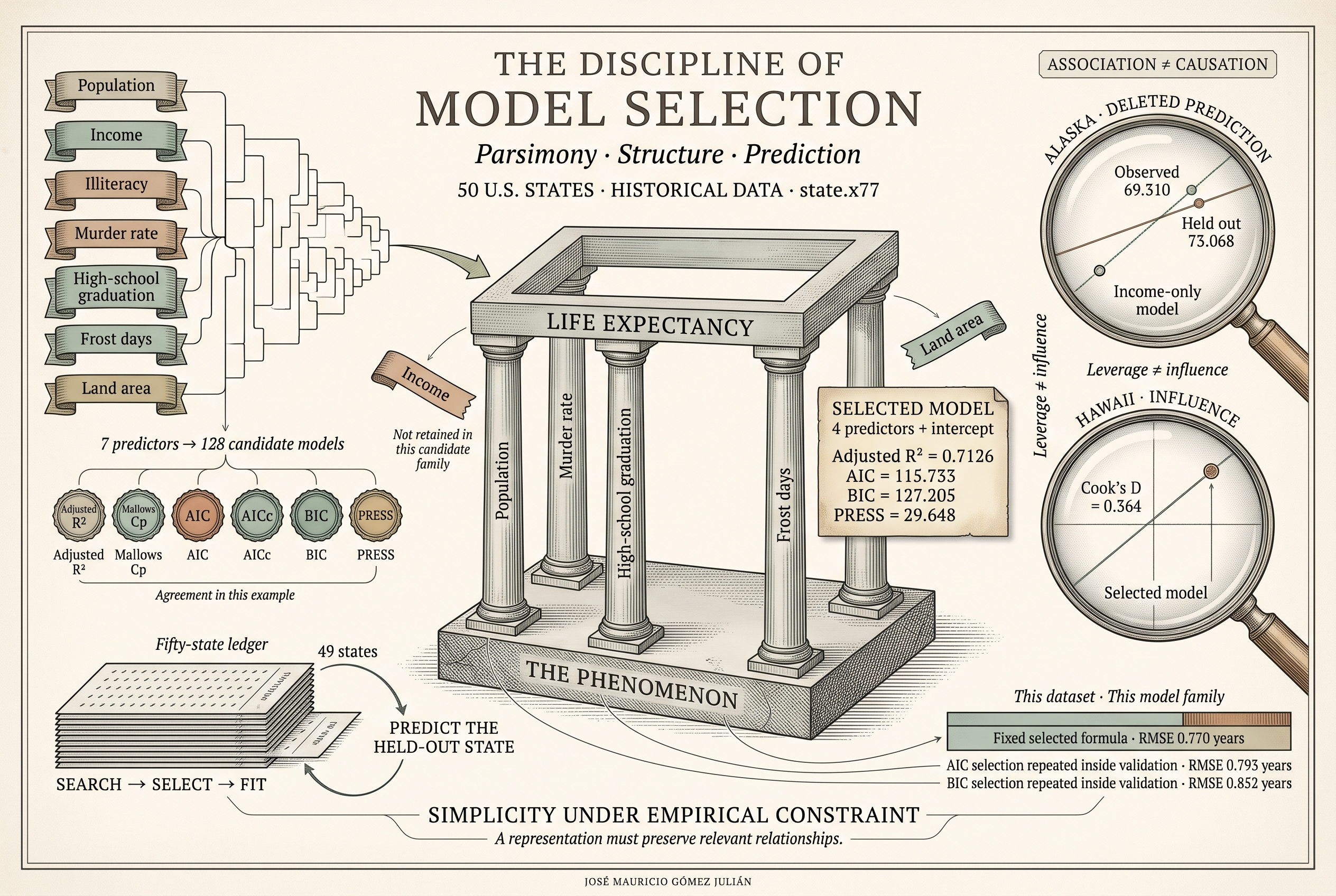
Seven numeric predictors and a mandatory intercept produce 2⁷ = 128 subsets, including the intercept-only model; 127 contain at least one predictor. This family excludes interactions, polynomials, and additional transformations. Its best candidate is therefore best within that universe, not among every conceivable representation.
Branch-and-bound can locate best subsets by size without naively fitting every combination. However, the returned table depends on how many candidates per size are requested. leaps() and regsubsets() are search tools; choosing a size and evaluating the result remain additional decisions. Nor does retaining only the lowest RSS per size guarantee the minimum PRESS, which also depends on leverage. All 128 candidates were fitted here to check every criterion (Lumley, n.d.).
| # | Predictors | p | R̄² | Cₚ | AIC | BIC | PRESS |
|---|---|---|---|---|---|---|---|
| 1 | pop + murder + hsgrad + frost | 5 | 0.7126 | 2.020 | 115.733 | 127.205 | 29.648 |
| 2 | pop + income + murder + hsgrad + frost | 6 | 0.7061 | 4.009 | 117.720 | 131.104 | 31.322 |
| 3 | pop + illiteracy + murder + hsgrad + frost | 6 | 0.7061 | 4.013 | 117.724 | 131.108 | 31.053 |
| 4 | pop + murder + hsgrad + frost + area | 6 | 0.7060 | 4.018 | 117.731 | 131.115 | 34.284 |
| 5 | murder + hsgrad + frost | 4 | 0.6939 | 3.740 | 117.974 | 127.534 | 31.197 |
| 6 | income + murder + hsgrad + frost | 5 | 0.6894 | 5.411 | 119.614 | 131.086 | 32.695 |
| 7 | illiteracy + murder + hsgrad + frost | 5 | 0.6892 | 5.430 | 119.634 | 131.107 | 32.721 |
| 8 | pop + income + illiteracy + murder + hsgrad + frost | 7 | 0.6993 | 6.002 | 119.712 | 135.008 | 32.953 |
The model containing pop + murder + hsgrad + frost maximizes adjusted R² and minimizes Cp, AIC, AICc, BIC, and PRESS. It has p = 5 regression coefficients and K = 6 parameters including variance. Its values are RSS = 23.308; R² = 0.7360; adjusted R² = 0.7126; AICc = 117.686; and Cp = 2.020. Agreement among six criteria is a feature of this example, not a general equivalence.

The three-predictor candidate murder + hsgrad + frost has BIC = 127.534, only 0.330 above the minimum. This supports acknowledging uncertainty about whether population is needed rather than declaring a decisive victory. Adding income, illiteracy, or area barely reduces RSS while consuming additional parameters.
7. PRESS: prediction with one observation omitted
Let ei = yi − ŷi be the ordinary residual and hii the corresponding diagonal entry of H. When the formula stays fixed and deletion fits retain full rank, the prediction residual obtained by excluding observation i is:
PRESS = Σi=1ndi² ; RMSELOOCV = √(PRESS/n)
This identity avoids refitting the same model n times. PRESS sums squared prediction errors; dividing by n gives the LOOCV mean squared error, and taking its square root restores the response unit. If d is a column vector, dᵀd is its squared Euclidean norm, a scalar. It is not obtained by taking a determinant of d.
In the income-only model, Alaska has an observed life expectancy of 69.310 years and a fitted value of 72.275. When Alaska is excluded, its predicted response rises to 73.068 years. The ordinary residual is −2.965, hii = 0.210875, and the deleted residual is −3.758. The relevant error compares the prediction to the observed response, rather than subtracting the two predictions from each other (R Core Team, n.d.-d).

A high PRESS does not establish that a particular observation has greater influence. The statistic aggregates errors over all units and combines residuals with design geometry. Attributing influence to Alaska or another state requires individual quantities, such as Cook’s distance or changes in coefficients.
8. Compare models with visible results
The table combines specifications from the original exercise with the selected candidate. The original four predictors are population, income, illiteracy, and area. The selected four are population, murder, high-school graduation, and frost. Every value uses the same fifty observations and includes an intercept.
| Model | RSS | R̄² | PRESS | RMSE LOOCV |
|---|---|---|---|---|
| Intercept only | 88.299 | 0.0000 | 91.940 | 1.356 |
| Income | 78.076 | 0.0974 | 89.322 | 1.337 |
| Population + murder | 30.445 | 0.6405 | 34.066 | 0.825 |
| Original four | 55.602 | 0.3143 | 91.427 | 1.352 |
| Selected four | 23.308 | 0.7126 | 29.648 | 0.770 |
| Seven predictors | 23.297 | 0.6922 | 41.322 | 0.909 |

Compared with the selected model, the full model reduces RSS from 23.308 to 23.297, a negligible fitting improvement, but increases PRESS from 29.648 to 41.322. Additional terms can improve the description of the sample while worsening prediction. This does not establish that omitted variables lack historical, health-related, or causal relevance; within this model family and dataset, including them fails to improve the compared criteria.
9. Stepwise selection and partial tests
Forward selection starts with mandatory terms and adds candidates; backward elimination starts with a larger model and removes terms; bidirectional search allows both operations. These are local traversals of a model family. They can stop at different solutions and do not guarantee a global optimum. They should not be confused with Gaussian elimination, which solves linear systems rather than comparing specifications.
In this example, forward and backward AIC searches reach the same candidate as exhaustive search. The trajectories below use the numerical convention of AIC(). Printed step() tables have different absolute values, while preserving the differences and ordering here.
| Direction | Step | Terms | AIC |
|---|---|---|---|
| Backward | 0 | pop + income + illiteracy + murder + hsgrad + frost + area | 121.709 |
| 1 | pop + income + illiteracy + murder + hsgrad + frost | 119.712 | |
| 2 | pop + income + murder + hsgrad + frost | 117.720 | |
| 3 | pop + murder + hsgrad + frost | 115.733 | |
| Forward | 0 | 1 | 174.329 |
| 1 | murder | 129.285 | |
| 2 | murder + hsgrad | 123.968 | |
| 3 | murder + hsgrad + frost | 117.974 | |
| 4 | pop + murder + hsgrad + frost | 115.733 |
For a partial test between nested models, let q be the rank difference, RSSR the reduced model’s residual sum of squares, and RSSF that of the larger model, which has pF coefficients. Under the null that the removed block contributes nothing and classical Gaussian assumptions:
A large F indicates greater loss of fit under the restriction. The p-value is the probability, under H₀ and the assumptions, of a statistic at least as extreme; it is not the probability that H₀ is true. drop1(model, test = "F") tests each term against the current model. A factor with several categories may involve multiple coefficients. For one coefficient, F = t² and the F-test and two-sided t-test p-values agree.
Removing terms with large p-values is an exploration rule, not proof of irrelevance. A threshold of α = 0.15 needs justification, and repeated tests do not automatically preserve a global Type I error rate of 0.15. Under AIC or BIC, a search proceeds while the criterion decreases; the aim is not to increase AIC. In step(), k = 2 gives AIC, while k = log(n) gives the BIC-penalized search (R Core Team, n.d.-a, n.d.-b).
10. Coefficients and diagnostics answer different questions
The selected model estimates the following conditional mean, in years. Population is measured in thousands of people; high-school graduation in percentage points; murder per 100,000 residents; and frost in days.
+ 0.04658·hsgrad − 0.005943·frost
| Term | β̂ | SE | t | p-value |
|---|---|---|---|---|
Intercept | 71.02713 | 0.95285 | 74.542 | < 0.0001 |
pop | 0.0000501 | 0.0000251 | 1.996 | 0.0520 |
murder | -0.30015 | 0.03661 | -8.199 | < 0.0001 |
hsgrad | 0.04658 | 0.01483 | 3.142 | 0.0030 |
frost | -0.00594 | 0.00242 | -2.455 | 0.0180 |
Holding other covariates fixed, a ten-percentage-point difference in graduation is associated with 0.466 years in the fitted mean. This is not an educational policy effect. Population’s p-value is about 0.052 even though AIC retains it; different decision rules can disagree without a logical contradiction.
In diagnostics, leverage describes location in predictor space; an outlying residual describes vertical discrepancy; and influence describes how much the fit changes when an observation is removed. High hii alone does not establish influence. Internally and externally studentized residuals differ as follows:
s²(i) = [RSS − ei²/(1 − hii)]/(n − p − 1)
ti = ei/[s(i)√(1 − hii)]
With a fixed formula, independent normal errors, and constant variance, ti follows a t distribution with n − p − 1 degrees of freedom. This supports observation diagnostics; it is not the justification for the t-test on β. Cook’s distance combines residual size and leverage to assess influence:
| State | hᵢᵢ | tᵢ | Cook D |
|---|---|---|---|
| Hawaii | 0.2398 | 2.543 | 0.3638 |
| Washington | 0.1717 | -1.490 | 0.0896 |
| Maine | 0.0642 | -2.201 | 0.0613 |
| South Carolina | 0.1029 | -1.646 | 0.0599 |
| Arizona | 0.1443 | -1.308 | 0.0568 |

Hawaii has the largest Cook’s D (0.364), followed by Washington. This calls for contextual examination and sensitivity analysis, not deleting states to improve the result. Selected-model VIFs range from 1.190 to 1.728, giving no indication of severe collinearity among these four predictors. They do not establish correct specification. Functional form, residual spread, normal quantiles, and geographic dependence also require examination; a set of plots does not certify every assumption.
11. Validate the selection procedure
LOOCV for a formula chosen using all data does not reproduce a procedure that first selects and then predicts. The omitted observation’s response has already affected the initial selection. To evaluate the procedure, exclude each state before selecting: fit all 128 candidates on the remaining 49, choose the minimum AIC or BIC, and predict the held-out state. Aggregate the fifty errors. When internal selection uses validation to tune hyperparameters, an additional inner loop is required; here internal choice uses an information criterion.
| Procedure | Sum of squared errors | RMSE, years |
|---|---|---|
| Formula selected on all data, followed by LOOCV | 29.648 | 0.770 |
| Exhaustive AIC selection within each partition | 31.476 | 0.793 |
| Exhaustive BIC selection within each partition | 36.255 | 0.852 |
Although AIC and BIC choose the same formula using all fifty states, their procedures have different errors when retrained. The decision path matters. These values describe a leave-state-out experiment within this candidate family; they establish neither universal AIC superiority nor performance in future years.
Stability can also be summarized by counting inclusions across the fifty training sets. Under AIC, population, murder, and graduation appear in 50/50; frost appears in 49/50. Under BIC, population appears in 38/50, murder and graduation in 50/50, and frost in 49/50. Income, illiteracy, and area never appear. These are local sensitivity frequencies under single-unit deletion, not posterior inclusion probabilities or independent population resamples.
Cawley and Talbot (2010) demonstrate that optimizing an estimated criterion can overfit model selection itself. Consequently, imputation, standardization, learned transformations, and term choice should occur within the relevant training set. Choosing between AIC, BIC, and other strategies after inspecting these outer results introduces another selection layer requiring independent evaluation.
12. Bayesian complexity: evidence, BIC, and DIC
A Bayesian model M specifies a likelihood p(y | θ, M) and a prior distribution p(θ | M). Marginal evidence integrates the likelihood with respect to that distribution:
Evidence averages fit over the allowed parameter space. It can therefore disfavor a flexible model that fits extremely well in a small region while assigning much of its prior mass to regions poorly compatible with the data. The Occam factor describes this effect under particular decompositions or approximations; it should not simply be equated with K log(n). BIC approximates −2 log p(y | M), apart from lower-order terms, under asymptotic and regularity assumptions. Priors matter and may require sensitivity analysis (Bishop, 2006).
DIC uses the posterior distribution. In the formulation of Spiegelhalter et al. (2002), effective complexity pD compares posterior mean deviance with deviance evaluated at the posterior mean:
pD = E[D(θ) | y] − D(E[θ | y])
DIC = E[D(θ) | y] + pD
Its relationship to AIC does not make DIC foreign to Bayesian analysis, nor identical to BIC. Interpretation can be problematic with multimodal posteriors, unsuitable parameterizations, or latent structures. Difficulty constructing a universal complexity measure does not imply absence of mathematical definitions or impossibility of formalization in set theory.
The published discussion remains instructive. Brooks questions the posterior summary; Smith examines priors and compatible parameterizations; Plummer challenges parts of the justification; Robert and Titterington discuss data use. Nelder emphasizes reviewing distribution, link, and predictor; Atkinson stresses diagnostics. These are specific, varied objections, not a single refutation of all Bayesian inference.
The stack loss example in that discussion illustrates a broader issue: an observation can appear outlying under one specification and cease to do so after a justified change of family or link. Removing observations is not always the answer. Selecting columns is only one part of selecting structure.
WAIC and LOO cross-validation provide other tools for Bayesian predictive evaluation, each with conditions and diagnostics. Vehtari et al. (2017) study their computation and assessment. This article does not fit a Bayesian model or calculate DIC or WAIC for the states: these concepts are introduced to distinguish problems rather than treat different criteria as one universal scale.
13. Alternatives and extensions
Discrete selection changes a formula abruptly: a coefficient stays or disappears. Regularization controls complexity gradually. Ridge shrinks coefficients with a quadratic penalty; lasso can produce exact zeros with an absolute-value penalty; elastic net combines both. The intercept is usually unpenalized. Predictor scales and the choice of λ matter (Friedman et al., 2010).
+ λ[α Σj≥1|βj| + (1 − α)Σj≥1βj²/2] }
Setting α = 0 gives ridge and α = 1 gives lasso. Choosing λ or α belongs inside training for each outer evaluation. Standardization must also be estimated there. With correlated predictors, inclusion stability can remain limited; penalization neither identifies causes nor fixes measurement problems.
Other extensions include sets of plausible models, predictive averaging, additive models for justified curvature, regional effects, and validation in geographic blocks. Specialized methods exist for post-selection inference, but validity depends on the procedure and target; applying ordinary intervals to the winner is insufficient. For a confirmatory question, prespecification or independent inference data may be preferable.
Once factors, interactions, or spline bases are introduced, selecting variables and selecting columns no longer coincide. A categorical variable can occupy several columns; an interaction may require retaining lower-order terms. Search should operate on blocks and restrictions consistent with the scientific meaning of the terms.
14. A reasoned selection protocol
- Define purpose and unit of analysis. Specify whether the target is association, prediction, or a causal effect, and the population or situation of intended generalization.
- Audit measurement and timing. Examine units, missingness, errors, predictor availability, and dependence among observations.
- Delimit candidates and restrictions. Justify mandatory terms, blocks, interactions, and transformations before evaluating results.
- Compare against a simple reference. Use the same observations, a common parameter-counting convention, and compatible criteria.
- Validate the entire procedure. Repeat selection and learned transformations inside training; reserve outer evaluation.
- Assess diagnostics and stability. Examine residuals, influence, functional form, and sensitivity to reasonable decisions.
- Interpret with explicit scope. Distinguish association from mechanism, acknowledge selection uncertainty, and document limitations.
For the fifty states, four predictors provide a favorable fit–prediction compromise within the additive family studied. Agreement among criteria, the nearby three-variable candidate, and different AIC/BIC stability patterns should be communicated together. The scientific result is more than a winning formula: it includes its scope, the decisions that produced it, and the conditions that might require revision.
Rigorous selection preserves relevant relationships, checks consequences, and makes the uncertainty of reduction visible.
Appendix A. Complete code and checks
The following script reproduces the search, tables, estimates, direct PRESS calculation, stepwise paths, VIFs, and evaluation with selection inside each training set. Its core uses only base R. The leaps block is optional and runs only if that package is installed. Variable names are identical in both languages to facilitate comparison.
It was executed in R 4.3.3, and the principal quantities were also checked through an independent QR calculation. Analytic PRESS was compared with explicit refits; stopifnot() checks detect unexpected numerical changes. No random simulation is involved. Article figures were generated from the same quantities; plot(chosen) supplies additional R diagnostics.
# Run blocks in their displayed order. All core calculations use base R.
base <- as.data.frame(datasets::state.x77)
names(base) <- c("pop", "income", "illiteracy", "life",
                 "murder", "hsgrad", "frost", "area")
xvars <- setdiff(names(base), "life")
stopifnot(nrow(base) == 50L, !anyNA(base))
subsets <- c(list(character(0)), unlist(lapply(seq_along(xvars), function(j) {
  combn(xvars, j, simplify = FALSE)
}), recursive = FALSE))
forms <- lapply(subsets, function(v) {
  if (length(v)) reformulate(v, response = "life") else life ~ 1
})
fits <- lapply(forms, lm, data = base)
full <- lm(life ~ ., data = base)
sigma2_full <- deviance(full) / df.residual(full)
score <- function(m, sigma2_ref = sigma2_full) {
  n <- nobs(m)
  p <- m$rank                  # regression coefficients, including intercept
  K <- attr(logLik(m), "df")   # p + residual variance for Gaussian lm
  press <- sum((residuals(m) / (1 - hatvalues(m)))^2)
  c(p = p, K = K, RSS = deviance(m),
    adjR2 = summary(m)$adj.r.squared,
    Cp = deviance(m) / sigma2_ref - n + 2 * p,
    AIC = AIC(m), BIC = BIC(m),
    AICc = AIC(m) + 2 * K * (K + 1) / (n - K - 1),
    PRESS = press, RMSEloo = sqrt(press / n))
}
tab <- as.data.frame(t(vapply(fits, score, numeric(10))))
tab$terms <- vapply(subsets, function(v) {
  if (length(v)) paste(v, collapse = " + ") else "Intercept only"
}, character(1))
stopifnot(nrow(tab) == 128L)
best_id <- which.min(tab$AIC)
chosen <- fits[[best_id]]
tab[order(tab$AIC), c("terms", "p", "adjR2", "Cp", "AIC", "BIC", "AICc", "PRESS")][1:8, ]
# All six criteria choose the same candidate in this particular search.
stopifnot(length(unique(c(best_id, which.min(tab$BIC),
  which.min(tab$AICc), which.min(tab$Cp), which.min(tab$PRESS),
  which.max(tab$adjR2)))) == 1L)
stopifnot(abs(deviance(chosen) - 23.308042796884) < 1e-8,
          abs(score(chosen)["PRESS"] - 29.648232954953) < 1e-8)

# Direct exhaustive search using leaps (optional; core code above needs no package).
if (requireNamespace("leaps", quietly = TRUE)) {
  search <- leaps::regsubsets(life ~ ., data = base,
                             nvmax = 7, nbest = 1, method = "exhaustive")
  summary(search)$which
  summary(search)$adjr2
}

# PRESS and the Alaska deletion example.
income_model <- lm(life ~ income, data = base)
i <- match("Alaska", rownames(base))
without_i <- lm(life ~ income, data = base[-i, , drop = FALSE])
c(observed = base$life[i], fitted = fitted(income_model)[i],
  heldout = predict(without_i, newdata = base[i, , drop = FALSE]),
  deleted = residuals(income_model)[i] / (1 - hatvalues(income_model)[i]))
press_fast <- sum((residuals(chosen) / (1 - hatvalues(chosen)))^2)
press_direct <- sum(vapply(seq_len(nrow(base)), function(i) {
  m <- lm(formula(chosen), data = base[-i, , drop = FALSE])
  (base$life[i] - predict(m, newdata = base[i, , drop = FALSE]))^2
}, numeric(1)))
stopifnot(isTRUE(all.equal(unname(press_fast), unname(press_direct), tolerance = 1e-10)))

# Stepwise candidates: same data, explicit scopes and directions.
lower <- lm(life ~ 1, data = base)
scope <- list(lower = formula(lower), upper = formula(full))
back_aic <- step(full, scope = scope, direction = "backward", trace = 0)
fwd_aic <- step(lower, scope = scope, direction = "forward", trace = 0)
back_bic <- step(full, scope = scope, direction = "backward",
                 k = log(nrow(base)), trace = 0)
drop1(full, test = "F")
add1(lower, scope = formula(full), test = "F")

# Estimates and diagnostics; conventional inference conditions on a fixed formula.
coef(summary(chosen))
confint(chosen)
diag_tab <- data.frame(state = rownames(base),
  leverage = hatvalues(chosen), rstudent = rstudent(chosen),
  Cook = cooks.distance(chosen),
  deleted = residuals(chosen) / (1 - hatvalues(chosen)))
diag_tab[order(-diag_tab$Cook), ][1:5, ]
selected_vars <- attr(terms(chosen), "term.labels")
vif <- vapply(selected_vars, function(v) {
  others <- setdiff(selected_vars, v)
  1 / (1 - summary(lm(reformulate(others, response = v), data = base))$r.squared)
}, numeric(1))
vif
# Optional plotting in an interactive R session:
# par(mfrow = c(2, 2)); plot(chosen); par(mfrow = c(1, 1))

# Outer leave-one-state-out validation of the entire exhaustive AIC/BIC search.
# No held-out response is used to choose the candidate in its training partition.
outer_errors <- matrix(NA_real_, nrow(base), 2,
                       dimnames = list(rownames(base), c("AIC", "BIC")))
inclusions <- matrix(0L, length(xvars), 2,
                     dimnames = list(xvars, c("AIC", "BIC")))
for (i in seq_len(nrow(base))) {
  train <- base[-i, , drop = FALSE]
  local_fits <- lapply(forms, lm, data = train)
  for (criterion in colnames(outer_errors)) {
    criterion_fun <- get(criterion, mode = "function")
    id <- which.min(vapply(local_fits, criterion_fun, numeric(1)))
    winner <- local_fits[[id]]
    outer_errors[i, criterion] <- base$life[i] -
      predict(winner, newdata = base[i, , drop = FALSE])
    v <- attr(terms(winner), "term.labels")
    inclusions[v, criterion] <- inclusions[v, criterion] + 1L
  }
}
colSums(outer_errors^2)
sqrt(colMeans(outer_errors^2))
inclusions
stopifnot(abs(sqrt(mean(outer_errors[, "AIC"]^2)) - 0.793422289702) < 1e-8,
          abs(sqrt(mean(outer_errors[, "BIC"]^2)) - 0.851525323981) < 1e-8)
# Local inclusion frequencies are sensitivity summaries, not posterior probabilities.
cat("All numerical checks passed.\n")
sessionInfo()
Appendix B. Data used
All fifty records are embedded below. English state names preserve correspondence with R row names. Units are specified in section 5.
View all 50 states and eight variables
| State | pop | income | illiteracy | life | murder | hsgrad | frost | area |
|---|---|---|---|---|---|---|---|---|
| Alabama | 3615 | 3624 | 2.1 | 69.05 | 15.1 | 41.3 | 20 | 50708 |
| Alaska | 365 | 6315 | 1.5 | 69.31 | 11.3 | 66.7 | 152 | 566432 |
| Arizona | 2212 | 4530 | 1.8 | 70.55 | 7.8 | 58.1 | 15 | 113417 |
| Arkansas | 2110 | 3378 | 1.9 | 70.66 | 10.1 | 39.9 | 65 | 51945 |
| California | 21198 | 5114 | 1.1 | 71.71 | 10.3 | 62.6 | 20 | 156361 |
| Colorado | 2541 | 4884 | 0.7 | 72.06 | 6.8 | 63.9 | 166 | 103766 |
| Connecticut | 3100 | 5348 | 1.1 | 72.48 | 3.1 | 56 | 139 | 4862 |
| Delaware | 579 | 4809 | 0.9 | 70.06 | 6.2 | 54.6 | 103 | 1982 |
| Florida | 8277 | 4815 | 1.3 | 70.66 | 10.7 | 52.6 | 11 | 54090 |
| Georgia | 4931 | 4091 | 2 | 68.54 | 13.9 | 40.6 | 60 | 58073 |
| Hawaii | 868 | 4963 | 1.9 | 73.6 | 6.2 | 61.9 | 0 | 6425 |
| Idaho | 813 | 4119 | 0.6 | 71.87 | 5.3 | 59.5 | 126 | 82677 |
| Illinois | 11197 | 5107 | 0.9 | 70.14 | 10.3 | 52.6 | 127 | 55748 |
| Indiana | 5313 | 4458 | 0.7 | 70.88 | 7.1 | 52.9 | 122 | 36097 |
| Iowa | 2861 | 4628 | 0.5 | 72.56 | 2.3 | 59 | 140 | 55941 |
| Kansas | 2280 | 4669 | 0.6 | 72.58 | 4.5 | 59.9 | 114 | 81787 |
| Kentucky | 3387 | 3712 | 1.6 | 70.1 | 10.6 | 38.5 | 95 | 39650 |
| Louisiana | 3806 | 3545 | 2.8 | 68.76 | 13.2 | 42.2 | 12 | 44930 |
| Maine | 1058 | 3694 | 0.7 | 70.39 | 2.7 | 54.7 | 161 | 30920 |
| Maryland | 4122 | 5299 | 0.9 | 70.22 | 8.5 | 52.3 | 101 | 9891 |
| Massachusetts | 5814 | 4755 | 1.1 | 71.83 | 3.3 | 58.5 | 103 | 7826 |
| Michigan | 9111 | 4751 | 0.9 | 70.63 | 11.1 | 52.8 | 125 | 56817 |
| Minnesota | 3921 | 4675 | 0.6 | 72.96 | 2.3 | 57.6 | 160 | 79289 |
| Mississippi | 2341 | 3098 | 2.4 | 68.09 | 12.5 | 41 | 50 | 47296 |
| Missouri | 4767 | 4254 | 0.8 | 70.69 | 9.3 | 48.8 | 108 | 68995 |
| Montana | 746 | 4347 | 0.6 | 70.56 | 5 | 59.2 | 155 | 145587 |
| Nebraska | 1544 | 4508 | 0.6 | 72.6 | 2.9 | 59.3 | 139 | 76483 |
| Nevada | 590 | 5149 | 0.5 | 69.03 | 11.5 | 65.2 | 188 | 109889 |
| New Hampshire | 812 | 4281 | 0.7 | 71.23 | 3.3 | 57.6 | 174 | 9027 |
| New Jersey | 7333 | 5237 | 1.1 | 70.93 | 5.2 | 52.5 | 115 | 7521 |
| New Mexico | 1144 | 3601 | 2.2 | 70.32 | 9.7 | 55.2 | 120 | 121412 |
| New York | 18076 | 4903 | 1.4 | 70.55 | 10.9 | 52.7 | 82 | 47831 |
| North Carolina | 5441 | 3875 | 1.8 | 69.21 | 11.1 | 38.5 | 80 | 48798 |
| North Dakota | 637 | 5087 | 0.8 | 72.78 | 1.4 | 50.3 | 186 | 69273 |
| Ohio | 10735 | 4561 | 0.8 | 70.82 | 7.4 | 53.2 | 124 | 40975 |
| Oklahoma | 2715 | 3983 | 1.1 | 71.42 | 6.4 | 51.6 | 82 | 68782 |
| Oregon | 2284 | 4660 | 0.6 | 72.13 | 4.2 | 60 | 44 | 96184 |
| Pennsylvania | 11860 | 4449 | 1 | 70.43 | 6.1 | 50.2 | 126 | 44966 |
| Rhode Island | 931 | 4558 | 1.3 | 71.9 | 2.4 | 46.4 | 127 | 1049 |
| South Carolina | 2816 | 3635 | 2.3 | 67.96 | 11.6 | 37.8 | 65 | 30225 |
| South Dakota | 681 | 4167 | 0.5 | 72.08 | 1.7 | 53.3 | 172 | 75955 |
| Tennessee | 4173 | 3821 | 1.7 | 70.11 | 11 | 41.8 | 70 | 41328 |
| Texas | 12237 | 4188 | 2.2 | 70.9 | 12.2 | 47.4 | 35 | 262134 |
| Utah | 1203 | 4022 | 0.6 | 72.9 | 4.5 | 67.3 | 137 | 82096 |
| Vermont | 472 | 3907 | 0.6 | 71.64 | 5.5 | 57.1 | 168 | 9267 |
| Virginia | 4981 | 4701 | 1.4 | 70.08 | 9.5 | 47.8 | 85 | 39780 |
| Washington | 3559 | 4864 | 0.6 | 71.72 | 4.3 | 63.5 | 32 | 66570 |
| West Virginia | 1799 | 3617 | 1.4 | 69.48 | 6.7 | 41.6 | 100 | 24070 |
| Wisconsin | 4589 | 4468 | 0.7 | 72.48 | 3 | 54.5 | 149 | 54464 |
| Wyoming | 376 | 4566 | 0.6 | 70.29 | 6.9 | 62.9 | 173 | 97203 |
References
Akaike, H. (1974). A new look at the statistical model identification. IEEE Transactions on Automatic Control, 19(6), 716–723. https://doi.org/10.1109/TAC.1974.1100705
Bishop, C. M. (2006). Pattern recognition and machine learning. Springer. https://www.microsoft.com/en-us/research/publication/pattern-recognition-machine-learning/
Cawley, G. C., & Talbot, N. L. C. (2010). On over-fitting in model selection and subsequent selection bias in performance evaluation. Journal of Machine Learning Research, 11, 2079–2107. https://jmlr.org/papers/v11/cawley10a.html
Friedman, J., Hastie, T., & Tibshirani, R. (2010). Regularization paths for generalized linear models via coordinate descent. Journal of Statistical Software, 33(1), 1–22. https://doi.org/10.18637/jss.v033.i01
Hurvich, C. M., & Tsai, C.-L. (1989). Regression and time series model selection in small samples. Biometrika, 76(2), 297–307. https://doi.org/10.1093/biomet/76.2.297
Kutner, M. H., Nachtsheim, C. J., Neter, J., & Li, W. (2005). Applied linear statistical models (5th ed.). McGraw-Hill/Irwin.
Lumley, T. (n.d.). leaps: Regression subset selection [Package manual]. https://cran.r-universe.dev/leaps/doc/manual.html
Mallows, C. L. (1973). Some comments on Cp. Technometrics, 15(4), 661–675. https://doi.org/10.1080/00401706.1973.10489103
Marx, K. (1999). Capital (Vol. III, Chap. 48, “The trinity formula”). Marxists Internet Archive. (Original work published 1894). https://www.marxists.org/archive/marx/works/1894-c3/ch48.htm
R Core Team. (n.d.-a). Add or drop all possible single terms to a model [Documentation]. https://stat.ethz.ch/R-manual/R-devel/library/stats/html/add1.html
R Core Team. (n.d.-b). Choose a model by AIC in a stepwise algorithm [Documentation]. https://stat.ethz.ch/R-manual/R-devel/library/stats/html/step.html
R Core Team. (n.d.-c). Extract AIC from a fitted model [Documentation]. https://stat.ethz.ch/R-manual/R-devel/library/stats/html/extractAIC.html
R Core Team. (n.d.-d). Regression deletion diagnostics [Documentation]. https://stat.ethz.ch/R-manual/R-devel/library/stats/html/influence.measures.html
R Core Team. (n.d.-e). US state facts and figures [Dataset documentation]. https://stat.ethz.ch/R-manual/R-devel/library/datasets/html/state.html
Schwarz, G. (1978). Estimating the dimension of a model. The Annals of Statistics, 6(2), 461–464. https://doi.org/10.1214/aos/1176344136
Spiegelhalter, D. J., Best, N. G., Carlin, B. P., & van der Linde, A. (2002). Bayesian measures of model complexity and fit. Journal of the Royal Statistical Society: Series B (Statistical Methodology), 64(4), 583–639. https://doi.org/10.1111/1467-9868.00353
Vehtari, A., Gelman, A., & Gabry, J. (2017). Practical Bayesian model evaluation using leave-one-out cross-validation and WAIC. Statistics and Computing, 27, 1413–1432. https://doi.org/10.1007/s11222-016-9696-4
Leave a Comment/Deja un Comentario