You can also find this library at CRAN and download it directly from R and RStudio.

LISTEN TO THIS POST AS A PODCAST:

Nonlinear Dynamics · Symbolic Regression · ODE · SDE

What Equation Is Hiding in the Data? An Introduction to EmpiricalDynamics

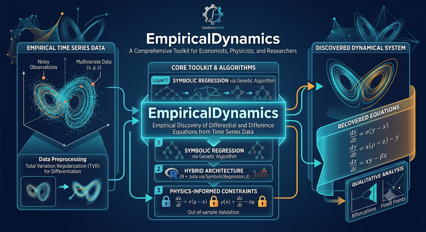
An R package for discovering and evaluating differential equations directly from time series, combining robust numerical differentiation, symbolic regression, stochastic modelling, temporal validation, and a high-performance Julia backend.

EmpiricalDynamics · R · Julia · SymbolicRegression.jl · development version 0.1.13 · developed by José Mauricio Gómez Julián · GitHub

Project status — August 2026. The main GitHub branch is currently at version 0.1.13 and declares GPL (≥ 3). The version currently published on CRAN is 0.1.9, which predates that licensing change.

We have a time series: a country’s GDP, a biological population, a temperature record, an interest rate, the concentration of a substance, or the reading of a sensor. We suspect that some dynamical law lies behind its motion. The problem is that we do not know what that law is.

One strategy is to choose an equation in advance and estimate its parameters. This is the familiar approach: assume linear, logistic, exponential, or some other known dynamics and ask which parameter values best fit the data.

EmpiricalDynamics also allows us to ask the inverse question: what functional form can the algorithm itself discover from the observed dynamics?

Instead of restricting the problem from the outset to \(\dot Z=\alpha+\beta Z\), a symbolic search can explore combinations of variables and mathematical operations, generate competing candidate equations, and compare their fit against their complexity.

The fundamental idea

The goal is not merely to predict the next observation with a black box. It is to recover an interpretable mathematical expression describing the observed dynamics and then subject that expression to diagnostics, simulations, and behavioural checks.

From estimating parameters to discovering equations

Suppose we already know the functional form:

\[ \frac{dZ}{dt} = \alpha+\beta Z. \]

Then the problem is essentially to estimate \(\alpha\) and \(\beta\).

Equation discovery poses a broader problem:

\[ \frac{dZ}{dt} = f(Z,\mathbf X;\boldsymbol{\theta}), \]

where we observe \(Z\) and possibly a set of exogenous variables \(\mathbf X\), but the function \(f(\cdot)\) itself is also unknown.

The algorithm must search simultaneously for a functional structure and its constants.

When the system is stochastic

Many real systems do not evolve according to a perfectly deterministic law. Even after discovering a systematic structure, a random component may remain whose intensity depends on the state of the system itself.

The natural description then moves from an ODE to a stochastic differential equation:

\[ dZ_t = f(Z_t,\mathbf X_t)\,dt + g(Z_t,\mathbf X_t)\,dW_t. \]

Here \(f\) is the drift: the systematic dynamics. \(g\) is the diffusion: the intensity of the stochastic component. \(W_t\) denotes a Wiener process.

Discovering an SDE therefore means solving two distinct problems: recovering the drift law and recovering the structure of the diffusion.

The architecture: six auditable stages

Preprocessing. Estimate numerical derivatives from potentially noisy observations.

Exploration. Examine relationships, phase portraits, surfaces, and possible nonlinearities before fitting.

Symbolic discovery. Search for candidate equations and construct a frontier trading goodness of fit against complexity.

Residual analysis. Ask what structure remains unexplained and, when appropriate, construct the diffusion term of an SDE.

Validation. Use time-aware cross-validation, trajectory simulation, and qualitative analysis of the dynamics.

Output. Produce LaTeX equations, tables, figures, and reports suitable for documentation or publication.

The first bottleneck: estimating a derivative without amplifying noise

To discover \[ \dot Z=f(Z,X) \] we first need an estimate of \(\dot Z\).

But numerical differentiation of noisy observations is dangerous: differentiation amplifies precisely the high-frequency fluctuations that we often want to treat as measurement noise.

EmpiricalDynamics provides several alternatives.

Method	Idea	Natural use case
TVR	Regularizes the total variation of the derivative.	Noisy data, trends, and possible discontinuities.
Savitzky–Golay	Uses local polynomial fits.	Relatively smooth signals where preserving peaks matters.
Smoothing spline	Smooths the series continuously before differentiating.	Smooth processes observed with noise.
Finite differences	Uses direct local numerical approximations.	Clean, sufficiently dense observations.
Spectral	Differentiates in the frequency domain.	Periodic signals; requires care with Gibbs phenomena.

TVR: smoothing the derivative without erasing all the structure

The method recommended by the documentation for many empirical applications is Total Variation Regularization.

Schematically, it seeks:

\[ \widehat{\dot Z} = \arg\min_{\dot Z} \left\| Z-\int_0^t \dot Z(\tau)\,d\tau \right\|_2^2 + \lambda \left\| \Delta\dot Z \right\|_1. \]

The first term forces the estimated derivative to reconstruct the observed series adequately. The second penalizes an excessively irregular derivative.

The current implementation internally rescales the optimization problem to improve numerical conditioning and uses a cascade of solvers:

1. CLARABEL

Currently the preferred TVR solver and the first option in the solver cascade.

2. SCS

Provides an alternative algorithmic family when the first solver does not achieve the desired status.

3. OSQP

Acts as a third optimization route when the preceding alternatives do not provide a satisfactory solution.

Selecting \(\lambda\)

select_lambda_cv_tvr() can automatically evaluate a grid of candidate values while reporting solver-convergence status.

The internal SDE paradox: a better drift can destroy the evidence for diffusion

This is perhaps the most interesting statistical idea in the package’s design.

TVR improves drift estimation precisely by smoothing. But the diffusion component of an SDE manifests itself to a large extent through high-frequency fluctuations.

If we then use the residuals of a strongly regularized derivative to recover \(g\), we may already have removed much of the information that we were trying to measure.

The conflict

TVR wants to clean high-frequency variation in order to estimate the drift. Diffusion lives precisely in that high-frequency variation. A method that improves the first task can therefore damage the second.

The solution: estimate diffusion from quadratic variation

When TVR is used, the current implementation recommends recovering diffusion not from TVR residuals but by returning to the observed increments themselves.

For an SDE:

\[ \frac{(\Delta Z)^2}{\Delta t} \approx g^2(X) + O(\Delta t). \]

estimate_diffusion_qv() uses this quadratic-variation relationship.

The estimate of \(g\) therefore no longer depends on residuals that TVR has already smoothed.

Individual values of \((\Delta Z)^2/\Delta t\) are naturally very noisy, so the procedure internally applies a rolling-median smoother before fitting the functional relationship.

The recovery tests reveal the problem directly

Historical configuration	Drift \(R^2\)	Diffusion \(R^2\)
Earlier solver + residual-based diffusion	0.864	0.591
Rescaled OSQP + residuals	0.887	0.070
Rescaled CLARABEL + residuals	0.841	0.005
CLARABEL + quadratic variation	0.841	0.985

The point is not that a “worse” solver happened to be better. It is exactly the opposite: as derivative estimation became more effective at removing high-frequency fluctuation, a diffusion estimate based on those residuals lost the signal it needed.

Returning to the raw increments allows the two problems to be decoupled.

The heart of the package: symbolic regression

Once the derivative has been estimated, the algorithm can search for expressions capable of explaining its behaviour.

Rather than optimizing constants alone, the search also changes the structure of the expressions themselves:

\[ Z,\quad Z^2,\quad XZ,\quad \sin(X),\quad e^Z,\quad \frac{X}{Z},\quad \ldots \]

The result should not be interpreted simply as “the equation with the smallest error.”

EmpiricalDynamics constructs a Pareto frontier containing equations that embody different trade-offs between fit and complexity.

Available criteria for choosing among candidates include AIC, BIC, and MDL, along with selection mechanisms operating directly on the frontier.

search_result <- symbolic_search(
  data = data,
  response = "dZ",
  predictors = c("Z", "X"),
  backend = "r_genetic",
  max_complexity = 15,
  n_generations = 50,
  population_size = 100,
  n_runs = 3
)

plot_pareto_front(search_result)

best_eq <- select_equation(
  search_result,
  criterion = "bic"
)

If theory already gives you a form, there is no prize for ignoring it

The package does not present blind symbolic search as superior in every situation.

If theory supplies a specific functional form, the documentation recommends fitting that form directly with fit_specified_equation().

equation <- fit_specified_equation(
  "alpha + beta * Z + gamma * Z^2 + delta * X",
  data = data,
  derivative_col = "dZ",
  method = "levenberg-marquardt",
  start = list(
    alpha = 0,
    beta = 1,
    gamma = -0.01,
    delta = 0.5
  )
)

This is an important methodological distinction: discovery when we do not know the structure; direct estimation when we already have a structural hypothesis that we want to test.

Explore before you search

explore_dynamics() allows the user to inspect relationships visually before launching a symbolic search.

It currently compares linear, quadratic, and cubic forms for predictors, retaining the winning fit, its coefficients, the range over which it was estimated, and the AIC values of the competing models.

This matters because a label such as “quadratic” does not tell us whether the fitted curve actually changes direction within the observed range.

A current caution

The Wiki itself reports that, in internal simulations, this AIC comparison classifies a truly linear relationship as “linear” only about 78% of the time. The label should therefore be read as model selection, not as infallible measurement of the true functional form.

Julia handles the heavy evolutionary search

The high-performance backend uses SymbolicRegression.jl.

The architecture keeps the statistical workflow, diagnostics, and user interface on the R side, while Julia can handle the more expensive, parallelizable evolutionary searches.

The file inst/julia/symbolic_backend.jl defines a scientific-search configuration controlling, among other things:

population size;
number of iterations;
maximum complexity;
parsimony penalties;
allowed operators;
checkpoints;
and detection of selected physical constants.

The current backend recognizes \(\pi\), \(e\), \(\varphi\), \(g\), \(c\), \(h\), and \(k_B\) as candidate constants, including several simple transformations of them.

This makes it possible, for example, to recognize that a discovered numerical coefficient lies close to \(\pi\), rather than reporting only a decimal expansion with no interpretation.

Iterative GLS: the current version preserves the full fitting history

When conditional variance changes with the state, the package can refine the drift through an iterative GLS procedure.

Schematically:

\[ r_i^{(k)} = \dot Z_i – \widehat f^{(k-1)}(Z_i,X_i), \]

\[ w_i^{(k)} = \frac{1} {\widehat g^{(k)}(Z_i,X_i)^2}, \]

and those weights modify the next drift estimate.

Recent versions corrected a fundamental detail: the previous loop could fail to recognize its own convergence when constants in a symbolic equation appeared as numeric literals.

The current implementation requires both:

Objective stability

Weighted deviance must have stopped changing materially.

Functional stability

Predictions from two successive iterations must also have become sufficiently close.

The result also preserves converged, stop_reason, history, selected_iteration, selection scores, and excluded candidates.

By default, iteration selection uses blocked cross-validation with contiguous blocks and refitting of the constants.

Residuals are a question, not a wastebasket

After fitting an equation, whatever remains unexplained may contain information about model misspecification or unresolved stochastic structure.

residual_diagnostics() brings several tests together:

Test	What it examines
Ljung–Box	Remaining serial dependence.
ARCH-LM	Conditional heteroskedasticity.
Breusch–Pagan	Variance related to predictors.
Jarque–Bera	Departures from normality.
Runs test	Remaining non-random patterns.

Validating a temporal equation without letting it look into the future

A time series should not be validated as though its rows were interchangeable.

The current implementation supports block validation and rolling or sliding schemes. In rolling mode, observations used for training occur before the test window.

cv <- cross_validate(
  equation,
  data = data,
  response = "dZ",
  k = 5,
  method = "rolling",
  horizon = 4,
  window = "expanding"
)

This sounds obvious, but it was not true in earlier versions. Version 0.1.12 corrected a defect in which the rolling implementation could use observations occurring after the window it was supposed to validate.

Other issues were also corrected:

blocks now cover all rows instead of dropping trailing observations;
\(R^2\) is evaluated against the training-set mean rather than a mean computed after observing the test data;
folds whose refit fails no longer silently disappear from the average;
observation weights are preserved when each fold is refitted;
a GLM is refitted as a GLM rather than accidentally reverting to an ordinary Gaussian regression.

An important limitation of that cross-validation

There is still a subtlety that the current documentation makes explicit.

When the response variable is a numerically estimated derivative, \(\dot Z_t\) itself may have been constructed using neighbouring observations.

With TVR, information from the entire series may even enter the derivative estimate.

Therefore, although the model in each rolling fold is not fitted using future observations under the corrected scheme, the derivative supplied to that model may previously have been calculated using such information.

What the CV means, then

The documentation explicitly warns that these scores can be used to compare candidate equations under the same preprocessing regime, but they should not be interpreted as the forecasting error we would expect on a completely new future series. The option intended to recompute the derivative within every fold, refit_derivative, is not yet implemented.

An equation must do more than fit points: it should behave correctly

EmpiricalDynamics includes tools for studying qualitative properties of a discovered equation:

fixed points;
stability;
bifurcations;
boundedness;
and full trajectory simulation.

This is an important difference between finding a flexible regression and recovering a plausible dynamical system.

Two expressions can have similar errors on the observed sample and still generate completely different dynamical portraits when integrated.

Bayesian bifurcations: a recent improvement

Version 0.1.11 substantially hardened analyze_bifurcations().

For models containing posterior draws, the function no longer automatically collapses all uncertainty into a single coefficient vector. It can sweep over the posterior distribution and return distributions of fixed points.

It also checks whether changing the bifurcation parameter actually changes the object’s predictions.

This prevents the function from producing a perfectly formatted but scientifically empty table in which every value of the bifurcation parameter gives exactly the same result because the substitution never reached the prediction mechanism.

Version 0.1.13 also added ed_derivative_step(), which officially exposes the \(10^{-6}\) central-difference step used in fixed-point classification.

Recovery tests: giving the algorithm a world whose law we already know

The most direct way to validate an equation-discovery algorithm is to construct a synthetic world in which the true law is known, hide that law from the algorithm, and ask whether it can recover it.

This does not prove causality in real observational data.

It does answer an indispensable prior question: if the true law is present in the data under controlled conditions, can the pipeline actually find it?

The Lorenz attractor

One benchmark uses the classical chaotic system:

\[ \frac{dx}{dt}=10(y-x), \]

\[ \frac{dy}{dt}=28x-xz-y, \]

\[ \frac{dz}{dt}=xy-\frac{8}{3}z. \]

Equation	\(R^2\) against the true dynamics
\(dx/dt\)	0.937
\(dy/dt\)	0.960
\(dz/dt\)	0.914
Average	0.937

The Wiki notes that these figures combine TVR differentiation error with symbolic-regression error, and that the evolutionary search itself is stochastic: different runs can return somewhat different results.

The stochastic benchmark

The second recovery test uses a deliberately challenging SDE:

\[ dZ_t = \left[ 10\sin(X_t)-2.5Z_t^3 \right]dt + \left[ 0.10+0.06|X_t| \right]dW_t. \]

With 5,000 observations, \(\Delta t=0.005\), and a documented SNR of approximately \(0.29\), the reported results are:

Component	\(R^2\)	RMSE	Procedure
Drift	0.841	0.547	TVR + iterative GLS
Diffusion	0.985	0.063	Quadratic variation

How to read these benchmarks

These are recovery tests on synthetic systems with known ground truth. They show that the pipeline can recover those structures under the conditions tested. They do not guarantee that an equation discovered from observational data is the true causal law of the system.

Discovering an equation is not the same as discovering causality

This boundary matters.

A symbolic expression can reproduce an observed relationship extremely well and still reflect omitted variables, confounding, simultaneity, measurement error, or a structure that works only within a particular regime.

Symbolic regression primarily answers: what mathematical structure is consistent with the observed dynamics?

Turning that structure into a causal claim requires additional information and reasoning.

Installation: CRAN or the development version

The version published on CRAN can be installed directly:

install.packages("EmpiricalDynamics")

To use the latest state of the repository:

remotes::install_github(
  "IsadoreNabi/EmpiricalDynamics"
)

The Julia backend can then be configured from R:

library(EmpiricalDynamics)

setup_julia_backend()

The package metadata currently declares R 4.0.0 or later and Julia 1.6 or later as the system requirement for the backend. The README currently recommends Julia 1.9 or later; using a recent Julia release satisfies both specifications.

The deeper methodological point

The temptation in equation discovery is to imagine a machine that receives a table and returns “the law of nature.”

EmpiricalDynamics becomes more interesting when understood in a different way.

Symbolic search is only one part of a much longer procedure.

First, we need a defensible derivative estimate. Then we explore the geometry of the relationship. Next, we search for or specify candidate equations. After that, we examine what remains in the residuals. If stochastic structure is present, drift and diffusion must be separated. Then we examine qualitative behaviour and simulate trajectories. Finally, we ask how much of the conclusion survives outside the immediate fit.

And every one of those steps can fail in a different way.

That is the most interesting contribution of EmpiricalDynamics: it does not treat equation discovery as a competition in which the expression with the highest \(R^2\) automatically wins. Instead, it treats it as a complete problem of dynamical inference. The equation should be parsimonious, survive diagnostics, reproduce qualitative properties, and correctly separate deterministic from stochastic structure. Its recovery tests show that the pipeline can rediscover known dynamics; its recent revisions show something equally important: when a metric, validation scheme, or bifurcation sweep did not mean exactly what it claimed to mean, the behaviour was audited and corrected. The final product is not simply a formula found by a computer. It is a more disciplined way of asking: what equation is genuinely consistent with the dynamics we observe, and what evidence do we have for believing it?

EmpiricalDynamics is developed by José Mauricio Gómez Julián. The current development branch declares GPL (≥ 3). The source code and change history are available on GitHub, while the mathematical documentation, recovery tests, and usage guides are available in the EmpiricalDynamics Wiki.