
Mathematical statistics · History of science
The Chi-Squared
Distribution
Foundations, Geometry, and Historical Origins
Originally published on September 10, 2021
Revised and expanded edition · October 29, 2026
Abstract
When does a discrepancy between observed and expected frequencies constitute evidence against a hypothesis? Answering this question requires constructing a measure of discrepancy and understanding its behavior under the proposed model. This essay reconstructs that connection, from Pearson’s criterion to quadratic forms in the multivariate normal distribution, ellipsoidal level sets, their transformation into spheres, and the radial integration that yields the chi-squared distribution. It distinguishes exact results from asymptotic approximations, develops the original examples, and provides reproducible R code.
A difference between what is observed and what is expected does not speak for itself. Its meaning depends on the variability of the process, the constraints on the data, and the sampling model. The chi-squared distribution connects these dimensions: it translates certain quadratic discrepancies into probabilities that we can interpret under explicit assumptions.
1. Two frequency problems
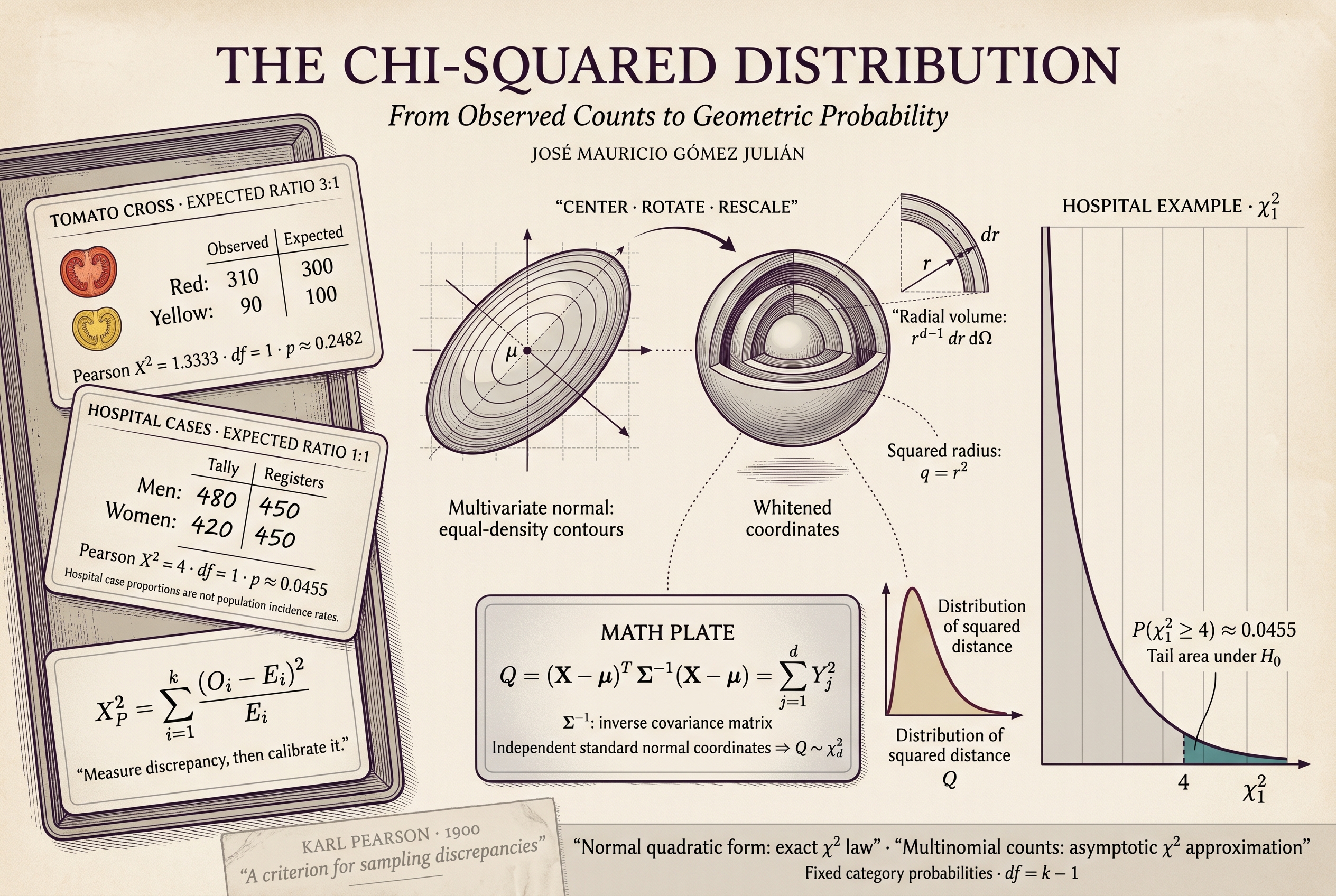
Snedecor and Cochran present two situations that capture the problem. A geneticist expects a particular tomato cross to produce red flesh and yellow flesh in a 3:1 ratio. Examining 400 fruits yields 310 red and 90 yellow. If the model were correct, the expected counts would be 300 and 100. Is the difference compatible with sampling fluctuation? [1]
In another example, 480 men and 420 women are observed among 900 hospitalized cases. Under the hypothesis of equal proportions, 450 cases would be expected in each category. How much weight should we attach to a deviation of thirty cases from the expected count?
Both problems require separating two operations: measuring discrepancy and calibrating its magnitude probabilistically. A positive number is not inferentially large or small without a reference distribution and degrees of freedom.
2. Pearson and the historical problem
Karl Pearson, a foundational figure in mathematical statistics and a communist, formulated a criterion for assessing whether a system of discrepancies could reasonably be attributed to random sampling. The central reference for this essay is his 1900 paper in The London, Edinburgh, and Dublin Philosophical Magazine and Journal of Science, volume 50, pages 157–175. This date refers to the cited publication; a reconstruction of its antecedents must distinguish it from other stages of development. [2]
The contribution connects a measure of deviation with a probability calculated under a hypothesis. It links the empirical problem, its mathematical representation, and the distribution of the statistic. The historical interest of the argument lies precisely in that transition.
Pearson’s political characterization is retained in the sense used in the original essay. His scientific contribution and the consistency of all his social positions are separate questions. The following exposition reconstructs the statistical argument; it does not assume that his ideological trajectory was uniform.
The 1900 text uses notation that is unfamiliar today. We therefore present a modern reconstruction and its connections with determinants, cofactors, and principal axes. The multivariate normal distribution provides the starting point for the geometry; the multinomial model will subsequently bring us back to frequencies.
3. Constructing a measure of discrepancy
Let Oi be the observed count and Ei the expected count in category i. With k categories, Pearson’s statistic adds their individual contributions:
Conceptual reading. Subtraction measures disagreement within each category. Squaring prevents positive and negative deviations from canceling and gives greater weight to large discrepancies. Dividing by the expected count weights the deviation according to the scale of the count. Finally, summation combines the individual discrepancies. Each included term requires Ei > 0.
The statistic is a finite sum, not an infinite series. The lower limit indicates where the sequence of terms begins and the upper limit where it ends. When all observed frequencies match their expected values, the statistic is zero. If at least one differs, it is positive.
Weighting by expected counts has a more precise justification than simply “accounting for sample size.” In count models, variability depends on the expected frequency. The multinomial structure introduces dependencies and a joint constraint; we will explain why this sum nevertheless acquires an approximate chi-squared law.
Conceptual reading. N is the total number of observations and pi the probability of the category under the hypothesis. Multiplying them gives the average count that would arise under repeated sampling. An expected count may be fractional even though every observed count is an integer.
Conceptual reading. Written in terms of proportions, the same formula shows that a fixed relative discrepancy receives more weight as N increases. More data can detect smaller deviations; statistical significance and substantive magnitude are therefore different concepts.
4. Variables, dimensions, and covariances
Before introducing matrices, distinguish three concepts. A deviation is the difference between a value and its reference. The standard deviation measures the dispersion of a variable. The standard error of a mean measures the dispersion of that mean across repeated samples.
Conceptual reading. If N observations are independent and have the same finite variance σ², the mean fluctuates less than an individual observation: its standard deviation is σ/√N. Under dependence, this expression must be modified to incorporate covariances. Here N counts observations, not dimensions.
In the geometric development, d denotes the number of components of a vector, N the sample size, and k the number of categories. A vector with d components lies in ℝd. Its effective degrees of freedom may be smaller when constraints apply.
Conceptual reading. Σ, uppercase sigma, is a d × d matrix recording the variability of each component and the covariation between pairs. Its diagonal contains variances. Other entries can be positive, negative, or zero. The symbol Σ is not the summation operator ∑.
A symmetric matrix for d components contains d variances and d(d−1)/2 distinct off-diagonal covariances. Counting those parameters does not change the dimension of the space containing each observation. Nor does it produce a space of dimension d(d−1).
Conceptual reading. R is the correlation matrix, and D contains the standard deviations, assumed positive. R describes associations without units; multiplying by D on both sides restores the original scales. This identity distinguishes a formulation using standardized variables from one using variables in their original units.
5. The quadratic form and the inverse
Suppose X has a multivariate normal distribution with population mean μ and positive definite population covariance matrix Σ. Its joint density can be written as follows. [3]
Conceptual reading. The density describes probabilistic concentration around x; integrating it over a region gives that region’s probability. The initial factor normalizes the total probability to one. |Σ| is the determinant, which adjusts the volume scale. The exponential decreases as the quadratic distance from the center increases. This is not a cumulative distribution function.
Conceptual reading. X−μ expresses displacement from the center. Σ−1 weights that displacement for dispersion and correlations. Transposition, denoted by ⊤, converts the first column vector into a row so that the product returns a scalar. Q is the squared Mahalanobis distance and has no units.
The exponent −1 denotes a matrix inverse: multiplying Σ by its inverse gives the identity matrix, the operation that leaves every vector unchanged. It does not represent a power of −1, subtraction, or alternating terms. The entries are not inverted separately either.
Conceptual reading. A deviation of ten units yields Q=25 when the standard deviation is two, and Q=0.25 when it is twenty. The same absolute displacement can be exceptional or ordinary depending on dispersion. In multiple dimensions, we must also adjust for the information shared by correlated variables.
Conceptual reading. z1 and z2 are deviations divided by their standard deviations; ρ is their correlation. The cross term adjusts for the joint direction of displacement. If ρ is positive, moving in the same direction in both variables is less unusual than moving in opposite directions. If ρ=0, Q reduces to the sum of the two squares. The negative sign in this expansion comes from matrix inversion, not an alternating series.
6. From historical to matrix notation
Pearson’s argument combines deviations, scales, and correlations. Its structure is now recognizable as a quadratic form. For standardized variables z, the relevant matrix is R, the correlation matrix; for unstandardized deviations, it is Σ. [2] [4]
Conceptual reading. Diagonal terms weight squared components. Cross terms incorporate relationships between components. Since the inverse matrix is symmetric, each pair appears twice in the full sum: aijzizj and ajizjzi. Combining them explains the factor 2. The condition i<j counts each pair once.
Conceptual reading. Deleting one row and one column produces a submatrix; its determinant is the minor Mij. The cofactor Cij introduces a positive sign when i+j is even and a negative sign when it is odd. Here an alternation of signs does occur, arising from the determinant’s structure. It must not be confused with the inverse exponent −1.
Conceptual reading. Transposing the cofactor matrix forms the classical adjugate and explains the interchange of indices. Dividing by a nonzero determinant completes the inversion. Minors and cofactors are not defined through elementary row operations, although those operations can help calculate determinants and inverses.
This translation preserves the algebraic content of the historical exposition while replacing less explicit summation symbols with defined limits. It also distinguishes an observed realization q from the random variable Q: fixing a value of the quadratic form defines a surface; allowing the vector to vary generates a distribution of values.
7. Ellipsoids, spheres, and topology
Conceptual reading. All points on this surface have the same squared Mahalanobis distance and the same normal density. Replacing equality with ≤ describes the interior together with its boundary. In two dimensions, the boundary is an ellipse; in three, it is an ellipsoidal surface. The bell-shaped density graph is a different object: it adds a further coordinate representing height.
Principal axes show the natural directions of dispersion. A noncircular ellipse has perpendicular major and minor axes centered at μ. In d dimensions, we choose d orthogonal directions. If some eigenvalues coincide, axes within the corresponding subspace are not unique, but an orthogonal choice is possible.
Conceptual reading. The columns of U are unit eigenvectors defining the principal directions. The positive eigenvalues λj are variances along those directions. At level c, each semiaxis has length √(cλj). The identity matrix I has ones on its diagonal and zeros elsewhere: it represents leaving a vector unchanged.
Conceptual reading. First subtract the center. U⊤ expresses the displacement in principal-axis coordinates. Λ−1/2 divides each coordinate by √λj, giving unit variance. Ellipsoids become spheres. Under normality, the coordinates of Y are independent standard normals: lack of correlation implies independence here because of the normality assumption.
Conceptual reading. The inverse transformation is x=μ+UΛ1/2y. Translation does not change volumes; an orthogonal matrix has a determinant with absolute value one; and the product of the factors √λj is |Σ|1/2. This factor cancels the determinant term in the density normalizer. Probabilities are preserved by jointly transforming the region, density, and volume element.
8. Radial integration and solid angles
In whitened coordinates, the density depends only on distance r from the origin. The probability of falling beyond a given radius is obtained by integrating over the entire exterior of a sphere, not over a single surface. Distinguishing radius from squared radius will be decisive.
Conceptual reading. r measures distance and q measures squared distance. The radius follows a chi distribution; its square follows a chi-squared distribution. We use r as the radial integration variable and q as the variable of the final distribution to keep their densities distinct.
Conceptual reading. A thin spherical shell has a volume approximately equal to its surface area times its thickness dr. Scaling the radius by a factor r scales its d−1 tangential directions by that factor, producing rd−1. dΩ captures directions on the unit sphere Sd−1. For d=2, the element is r dr dθ; for d=3, it is r² dr dΩ. In d=1 there are two directions, one on each half-line.
In three dimensions, a solid angle measures the area of a region’s radial projection onto the unit sphere; its unit is the steradian. The whole sphere spans 4π steradians. A face of a cube centered at the origin subtends 2π/3: its six faces divide spatial directions symmetrically. This is the geometric construction illustrated in the original document. In other dimensions, we speak of angular measure on the unit sphere. [6]
Conceptual reading. The numerator accumulates mass from the observed radius to infinity; the denominator normalizes by total radial mass. The angular integral and common constants cancel because all directions are included in both cases. This cancellation follows from radial symmetry and the same angular region, not from matching asymptotic behavior of eigenvectors.
These are volume integrals reduced using polar coordinates. They do not assign positive probability to a single surface of fixed radius: in this continuous model, that surface has probability zero. Probability mass occupies regions with radial thickness.
Conceptual reading. Changing the variable also changes the width of each interval. The factor 1/(2√q) adjusts for that change. Multiplying it by rd−1 produces the exponent d/2−1. This “minus one” comes from the Jacobian and the combination of powers; it does not indicate an alternating series either.
Conceptual reading. Γ is the function that supplies the density normalizer. It extends the factorial: for positive integers m, Γ(m)=(m−1)!. Substituting t=r²/2 in the total radial integral gives 2d/2−1Γ(d/2). The preceding ratio thus becomes a calculable, normalized probability.
9. The chi-squared law and its properties
Conceptual reading. The power term captures shell geometry and the change of variable; the exponential captures the decline of the normal density with distance. The denominator makes the integral over all positive values equal to one. This is a one-dimensional density, even though it arises from a d-dimensional problem.
We write Q ∼ χ²d: ∼ means “has distribution,” whereas = states equality between objects or expressions. In this derivation, d is a positive integer because it counts independent normal coordinates. The gamma family defines χ² distributions for any positive real number of degrees of freedom. [7]
Conceptual reading. Each squared standard normal contributes mean one and variance two. Summing d independent terms adds their means and variances. The gamma equivalence specifies scale two; under the rate parameterization, the rate is 1/2. Confusing rate and scale changes the model.
The support is [0,∞), although the density formula is stated for q>0. The density can diverge as q approaches zero when the degrees of freedom are less than two, without creating a point mass at zero. For d=2 it is exponential; increasing d makes it less asymmetric. A density can exceed one: it is integrated probability that must lie between zero and one.
Conceptual reading. The p-value is the probability, under H₀ and the model assumptions, of a statistic at least as discrepant as the observed one. Including or excluding the endpoint does not change this continuous integral. It is neither the probability that H₀ is true nor the probability that the result is “due to chance” in an absolute sense.
10. Why it works for counts
The preceding normal result is exact when its assumptions hold and population μ and Σ are used. Category counts are not exactly normal. Connecting them with χ² requires the multinomial model and a limiting argument.
Conceptual reading. Each independent observation belongs to exactly one category, the categories are exhaustive, and their probabilities remain constant across observations. The counts sum to N. Although individual observations are independent, counts in different categories are not: when one increases with the total fixed, less room remains for the others.
Conceptual reading. The fixed total induces negative dependence. This explains why it would be incomplete to justify Pearson’s statistic by assuming that each count has variance exactly equal to its expectation and that all counts are independent. That idea is natural under an independent Poisson model, but the multinomial requires incorporating the constraint on the total.
Conceptual reading. Once k−1 deviations are known, the total determines the remaining one. There are therefore only k−1 free directions, and the joint covariance matrix is singular in the full space. The relevant geometry lies in a subspace of dimension k−1.
Conceptual reading. W denotes the vector of Pearson residuals. Dividing by √(Npi) produces dimensionless residuals. Because the probabilities sum to one, s has unit length. The matrix I−ss⊤ removes direction s and leaves the k−1 directions orthogonal to it unchanged. It is a projection of rank k−1; the covariance identity is exact under the multinomial model.
With k fixed, fixed positive probabilities, and increasing N, the multinomial central limit theorem approximates these residuals by a normal vector in the free subspace. Choosing an orthonormal basis in that subspace gives k−1 independent standard normal coordinates. The sum of their squares yields the limit:
Conceptual reading. The arrow denotes convergence in distribution as N increases, not exact equality for every sample. This is the bridge between normal geometry and counts. Subtracting one reflects the constraint on the total rather than an arbitrary rule.
Conceptual reading. In regular goodness-of-fit problems, estimating m identifiable parameters can consume m additional directions. This formula requires appropriate estimation and regularity conditions, such as maximum likelihood based on the grouped counts. Mechanically subtracting parameters is insufficient: estimating them from ungrouped data before grouping can alter calibration. Structurally impossible categories also need specific treatment. [9]
11. The original examples, worked through
11.1. Tomatoes: a 3:1 ratio
The hypothesis specifies probabilities of 0.75 and 0.25. The 400 fruits are treated as independent observations under the model; clustering by plant or batch would require reassessing that assumption.
| Category | O | E | O − E | (O − E)²/E |
|---|---|---|---|---|
| Red flesh | 310 | 300 | 10 | 0.333333 |
| Yellow flesh | 90 | 100 | −10 | 1.000000 |
| Total | 400 | 400 | 0 | 1.333333 |
Conceptual reading. The absolute deviations are equal, but ten fruits carry more weight in a category with an expected count of one hundred than in one with an expected count of three hundred. With one degree of freedom, the approximate right-tail probability is 0.2482. At α=0.05, the 3:1 ratio is not rejected; this does not prove it is exactly true.
11.2. Hospital cases: a 1:1 ratio
| Category | O | E | O − E | (O − E)²/E |
|---|---|---|---|---|
| Men | 480 | 450 | 30 | 2 |
| Women | 420 | 450 | −30 | 2 |
| Total | 900 | 900 | 0 | 4 |
Conceptual reading. Under equal proportions, both categories contribute equally. The value 4 is not interpreted in isolation: with one degree of freedom, its right-tail probability is approximately 0.0455. At α=0.05, equal proportions are rejected within the model; at α=0.01, they are not. The significance level should be chosen before examining the result.
In the second example, the observed proportion of men is 480/900≈0.5333: about 3.33 percentage points above 0.5. This illustrates how a relatively small discrepancy can cross a conventional threshold. Its clinical or social relevance requires a substantive question and suitable data.
12. Applications, conditions, and limitations
Goodness of fit
This compares counts with specified probabilities. Categories must follow a clear definition; when continuous data are grouped, interval choices affect the result. Each interval’s probability must be calculated under the corresponding model. If parameters are estimated, the reference distribution requires justification.
Independence and homogeneity
In a table with r rows and c columns, independence states that joint probabilities factor into marginal probabilities. Homogeneity compares categorical distributions across populations or groups. Both can produce the same statistic, although their sampling designs differ.
Conceptual reading. Oi+ is the total for row i and O+j the total for column j. Their proportions estimate marginal probabilities under independence. The degrees-of-freedom formula accounts for the relevant constraints in an ordinary full table without structural zeros or other restrictions.
The count table contains observed values; expected values are calculated under the hypothesis. In R, xtabs() constructs the observed table, while chisq.test(... )$expected provides expected counts. Independence of observations does not follow from the independence that the test evaluates: it is a design assumption.
Conceptual reading. V summarizes the magnitude of association in a contingency table using the uncorrected Pearson statistic. It indicates neither direction nor causality; its interpretation depends on table structure and may benefit from bias corrections and intervals. In a 2 × 2 table, it equals the absolute value of φ. Residuals and proportions show which cells account for the association.
Variance of a normal population
The same distributional family appears in another problem with different assumptions: inference about a normal population variance.
Conceptual reading. For an independent sample from a normal population, S² uses N−1 in its denominator. Estimating the mean consumes one direction. Under H₀: σ²=σ₀², σ₀² is used in T. Depending on the alternative, the test can use the left tail, the right tail, or both; not every test based on χ² is therefore a right-tailed test. [10]
Diagnostics before calculation
- Observational unit: identify what is being counted and whether dependence, pairing, clustering, or repeated measurements are present.
- Counts: use frequencies rather than percentages without their sample size. Weighted frequencies from complex surveys may require design adjustments such as Rao–Scott corrections.
- Categories: they must be mutually exclusive and exhaustive under the model; structural zeros are not ordinary sampling zeros.
- Expected counts: inspect their magnitudes and distribution across cells. “All at least five” is a conservative rule of thumb, not a universal theorem or a condition on observed counts.
- Sparse data: consider an exact procedure, simulation consistent with the hypothesis, or scientifically justified pooling. Do not pool categories to obtain a desired result.
- Reporting: accompany the statistic with degrees of freedom, p-value, design, diagnostics, proportions, and a suitable measure of magnitude.
In 2 × 2 tables, Yates’s continuity correction modifies the approximation. R applies it by default in that case through chisq.test(), but it is not a universal remedy for sparse data. Fisher’s exact test and Monte Carlo methods use specific reference distributions. For tables, simulation in chisq.test() conditions on both margins, requires positive margins, and omits Yates’s correction; it does not automatically reproduce every sampling design. [11]
13. Reproduction and exploration in R
The code uses base R. RStudio can provide the working environment, but the functions belong to R. No external data files are required. The numerical outputs stated above are deterministic approximations; simulation experiments illustrate variability and depend on their replicates.
13.1. Manual calculation and the built-in test
# Original examples: probabilities fixed by H0.
# No parameters of the category probabilities have been estimated.
pearson_fixed <- function(observed, probabilities) {
  stopifnot(is.numeric(observed), is.numeric(probabilities),
            length(observed) == length(probabilities),
            length(observed) >= 2L,
            all(is.finite(observed)), all(observed >= 0),
            all(observed == floor(observed)), sum(observed) > 0,
            all(is.finite(probabilities)), all(probabilities > 0),
            abs(sum(probabilities) - 1) < 1e-10)
  expected <- sum(observed) * probabilities
  contributions <- (observed - expected)^2 / expected
  statistic <- sum(contributions)
  df <- length(observed) - 1L
  # Direct upper tail avoids subtracting a probability near 1 from 1.
  p_value <- pchisq(statistic, df = df, lower.tail = FALSE)
  automatic <- chisq.test(observed, p = probabilities)
  stopifnot(isTRUE(all.equal(statistic,
                            unname(automatic$statistic))),
            isTRUE(all.equal(p_value, automatic$p.value)))
  list(table = data.frame(observed, expected, contributions),
       X2 = statistic, df = df, p = p_value,
       test = automatic)
}
tomatoes <- pearson_fixed(c(red = 310, yellow = 90), c(0.75, 0.25))
hospital <- pearson_fixed(c(men = 480, women = 420), c(0.5, 0.5))
tomatoes$table
c(X2 = tomatoes$X2, df = tomatoes$df, p = tomatoes$p)
# X2 = 1.333333333; df = 1; p = 0.248213079
hospital$table
c(X2 = hospital$X2, df = hospital$df, p = hospital$p)
# X2 = 4; df = 1; p = 0.045500264

# Exact binomial alternatives: these are not Pearson approximations.
binom.test(310, 400, p = 0.75)
binom.test(480, 900, p = 0.5)
pchisq() returns cumulative probabilities; lower.tail = FALSE requests the upper tail. Given a vector of counts and probabilities, chisq.test() performs a goodness-of-fit test. The correct argument concerns 2 × 2 tables and does not change these vector-based tests. The checks compare manual summation with the built-in function.
13.2. An illustrative contingency table
The following table is an added example constructed to demonstrate the procedure; it is not part of the original data and does not represent an empirical study.
tab <- matrix(c(40, 20, 30, 50), nrow = 2, byrow = TRUE,
              dimnames = list(group = c("A", "B"),
                              response = c("Yes", "No")))
test <- chisq.test(tab, correct = FALSE)
test
test$observed
test$expected
test$residuals  # (O - E) / sqrt(E)
test$stdres     # Adjust for the variance of each residual.

X2_manual <- sum((tab - test$expected)^2 / test$expected)
df_manual <- (nrow(tab) - 1) * (ncol(tab) - 1)
p_manual <- pchisq(X2_manual, df = df_manual, lower.tail = FALSE)
V <- sqrt(X2_manual /
          (sum(tab) * min(nrow(tab) - 1, ncol(tab) - 1)))
c(X2 = X2_manual, df = df_manual, p = p_manual, V = V)
stopifnot(isTRUE(all.equal(p_manual, test$p.value)))

# Compare procedures: explicitly report which one is used.
chisq.test(tab, correct = TRUE)  # Yates, only for 2 x 2 tables.
fisher.test(tab)                # Fisher's exact test.
set.seed(20261029)
chisq.test(tab, simulate.p.value = TRUE, B = 99999)
With B=99,999 replicates, the smallest attainable simulated p-value is 1/(B+1)=0.00001. This resolution is not precision: the estimate retains Monte Carlo error. Standardized residuals help locate discrepancies, but assessing many cells requires considering multiplicity and dependence. [11]
13.3. From the normal distribution to χ²: checking the geometry
set.seed(20261029)
B <- 50000L
d <- 3L
Sigma <- matrix(c(4, 1, 0.5,
                  1, 2, 0.2,
                  0.5, 0.2, 1), nrow = d, byrow = TRUE)
# chol returns upper-triangular C with t(C) %*% C = Sigma.
C <- chol(Sigma)
Z <- matrix(rnorm(B * d), nrow = B, ncol = d)
X <- Z %*% C  # Each row has mean zero and covariance Sigma.
Q <- rowSums((X %*% solve(Sigma)) * X)
Q_standard <- rowSums(Z^2)
stopifnot(max(abs(Q - Q_standard)) < 1e-8)
c(empirical_mean = mean(Q), theoretical_mean = d,
  empirical_variance = var(Q), theoretical_variance = 2 * d)
hist(Q, breaks = 70, probability = TRUE,
     col = "#f5f0e8", border = "#d4c8b0",
     main = "Normal quadratic form and chi-squared law",
     xlab = "q")
curve(dchisq(x, df = d), add = TRUE, col = "#8b4513", lwd = 2)
# solve(Sigma) makes the inverse explicit for teaching purposes.
# For large problems, prefer factorizations and linear solves.
The identity between the two calculations of Q holds to numerical precision. By contrast, empirical means and variances only approximate their theoretical values because the simulation has finitely many replicates.
13.4. From counts to the asymptotic limit
set.seed(20261029)
B <- 30000L
prob <- c(0.2, 0.3, 0.5)
df <- length(prob) - 1L
threshold <- qchisq(0.95, df = df)
explore <- function(N) {
  O <- rmultinom(B, size = N, prob = prob)  # One sample per column.
  E <- N * prob
  residuals <- sweep(O, 1, E, "-")
  contributions <- sweep(residuals^2, 1, E, "/")
  X2 <- colSums(contributions)
  c(N = N, minimum_expected = min(E),
    mean = mean(X2), rejection_005 = mean(X2 > threshold),
    percentile_95 = unname(quantile(X2, 0.95)))
}
t(vapply(c(20L, 100L, 1000L), explore, numeric(5)))
qchisq(0.95, df = df)
# The mean of X2 is k - 1 even at finite N under this model.
# That does not make the chi-squared distribution exact.
# The percentile and rejection rate examine the approximation.

# Density, CDF, quantile, and random generation are distinct operations:
dchisq(4, df = 1)                       # Density height.
pchisq(4, df = 1, lower.tail = FALSE)  # Tail probability.
qchisq(0.95, df = 1)                    # 95th-percentile threshold.
rchisq(5, df = 1)                       # Five simulated values.
Simulation evaluates the procedure under a particular model; it does not guarantee validity for other designs. An approximation can improve with N while still exhibiting Monte Carlo fluctuation. The discreteness of counts also persists in a finite sample.
14. Synthesis and glossary
Discrepancy becomes interpretable evidence when its scale, constraints, and calibrating distribution are made explicit.
The journey began with observed and expected frequencies. The multivariate normal distribution represented discrepancy through a quadratic form with ellipsoidal levels. Centering, rotating, and rescaling produced standard normal coordinates; integrating over radial shells and squaring the radius yielded the χ² law. The multinomial model brought the argument back to counts and explained the asymptotic character of Pearson’s test.
This connection does not turn every quadratic deviation into a chi-squared variable, every geometric relationship into probabilistic equivalence, or every significant result into a causal conclusion. Its strength lies in showing how assumptions enable the transition between observation, mathematical structure, and inference.
| Symbol or concept | Meaning in this essay |
|---|---|
| N | Sample size or total count. |
| d | Dimension of the nondegenerate normal vector. |
| k | Number of categories in a goodness-of-fit test. |
| ν | Degrees of freedom of the reference distribution. |
| Σ / ∑ | Covariance matrix / summation operator. |
| Σ⁻¹ | Matrix inverse, existing under nonsingularity. |
| R / W | Correlation matrix / vector of Pearson residuals. |
| Q / q | Random quadratic variable / a value of that variable. |
| X²P | Pearson’s statistic for counts. |
| χ²ν | Family of distributions indexed by degrees of freedom. |
| r / q=r² | Radius / squared radius. |
| Density | Concentration whose integral over a region gives probability. |
| Homoscedasticity | Constancy or equality of variances within a model. |
| α / p-value | Nominal level of the procedure / tail probability under the hypothesis. |
| Diffeomorphism | A smooth bijection with a smooth inverse. |
15. References and the original paper
The original references are retained as part of the intellectual development. Added sources document the modern formulation and applications. The revised mathematical exposition is an explanatory reconstruction, not a verbatim transcription of the 1900 paper. The linked original essay is in Spanish; this English edition presents the revised argument in full.
- Snedecor, G. W., and Cochran, W. G. (1967). Statistical Methods, 6th ed. Iowa State University Press. See the introductory examples on pp. 20–21 cited in the original paper.
- Pearson, K. (1900). On the criterion that a given system of deviations from the probable in the case of a correlated system of variables is such that it can be reasonably supposed to have arisen from random sampling. Philosophical Magazine, series 5, 50(302), 157–175. DOI and publisher’s record.
- Penn State, STAT 505. Multivariate Normal Distribution. Multivariate normality, Mahalanobis distance, and ellipsoidal contours. Teaching materials.
- Boyd, S. (2007). Symmetric matrices, quadratic forms, matrix norm, and SVD. EE263, Stanford University. Teaching reference cited in the original. 2007–2008 course archive. See also Lall, S., Symmetric matrices and quadratic forms, EE263 notes.
- Gómez Julián, J. M. (2021; originally published under the name Isadore Nabi). Hacia una interpretación dialéctica-materialista de la topología general: génesis histórica-teórica de la topología desde la geometría y la teoría de conjuntos [Toward a dialectical-materialist interpretation of general topology: its historical and theoretical genesis from geometry and set theory]. The author’s essay, in Spanish. It contextualizes reflection on structural equivalences; probabilistic conditions are justified in the present text.
- Weisstein, E. W. Solid Angle. MathWorld, Wolfram Research. Consulted for the original essay in 2021. Definition and cube example.
- R Core Team. The (non-central) Chi-Squared Distribution,
statspackage documentation. Density, probabilities, quantiles, and simulation. - Kolmogorov, A. N. (1933). Grundbegriffe der Wahrscheinlichkeitsrechnung [Foundations of the Theory of Probability]. Springer. Historical reference added to contextualize the axiomatization of probability.
- NIST/SEMATECH. e-Handbook of Statistical Methods, §1.3.5.15, Chi-Square Goodness-of-Fit Test. Grouping, estimation, and degrees of freedom.
- NIST/SEMATECH. e-Handbook of Statistical Methods, §1.3.5.8, Chi-Square Test for the Variance. Testing a population variance.
- R Core Team. Pearson’s Chi-squared Test for Count Data,
statspackage documentation. chisq.test(), residuals, and Monte Carlo. - Wikipedia. Elipse [Ellipse]. Geometric source cited in the original and consulted there in 2021. Reference entry, in Spanish. Retained for traceability; the algebraic reconstruction relies on the teaching sources listed above.
The essay archive
The original version preserves the 2021 formulation and presentation in Spanish. This English page develops its examples, clarifies its notation, and expands the geometric and statistical foundations.
Read the original Spanish PDF ↗JOSÉ MAURICIO GÓMEZ JULIÁN · Marxist Philosophy of Science
History, geometry, and statistical inference
Leave a Comment/Deja un Comentario