
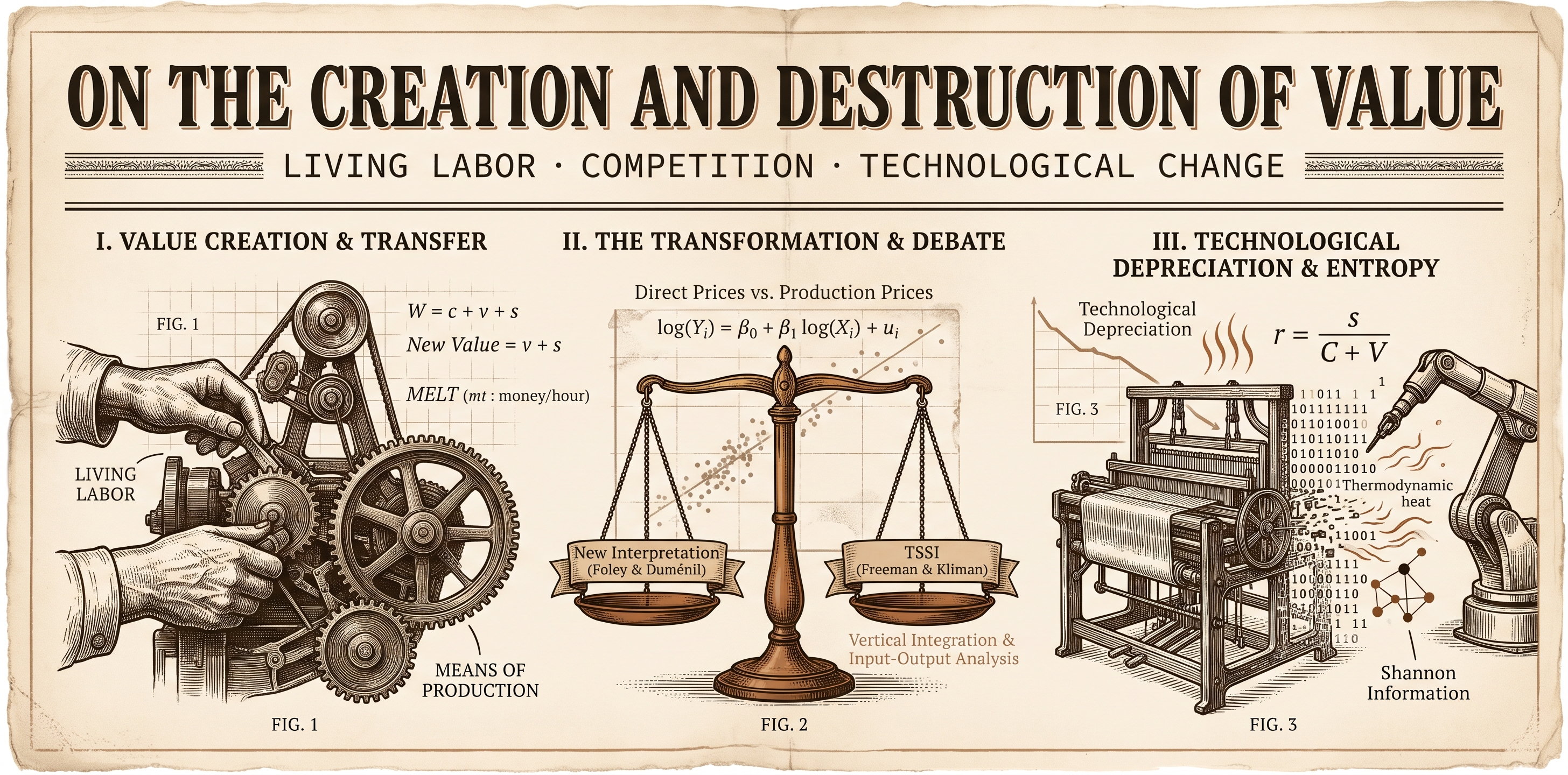
On the Creation
and Destruction of Value (Draft)
In Capitalist Political-Economic Systems in Particular and Economic Systems in General
An investigation of living labour, the means of production and technological devaluation. The essay examines controversies over values and prices, competition and profit rates, the temporality of models and vertical integration. It considers their historical and statistical foundations and explores the relations between value, energy and information. It includes the United States empirical appendix, all the graphic materials in the original document, and a reproducible methodological supplement.
Labour and the transformation of its own conditions
Labour produces commodities and transforms the conditions under which those commodities can be produced again. This relationship raises a decisive question: how can an activity that creates value also contribute, through technological development, to the devaluation of the means of production and products that it has itself made possible?
This essay examines that question by bringing together Marxian political economy, the history of economic thought, the epistemology of models, statistics and input–output analysis. Its starting point is the distinction between the creation of new value by living labour and the transfer of the value of the means of production. Its dynamic problem concerns changes in the social conditions of reproduction: a machine can remain physically operational yet lose value when a cheaper or more productive alternative appears.
The physical persistence of a means of production does not guarantee the persistence of its economic value.
The guiding proposition of this edition
The debate requires a distinction between the material conditions of the labour process and the social forms of production. Every society must reproduce its material existence; generalised commodity production, wage labour and the valorisation of capital belong to specific historical configurations. Extending the analysis to economic systems in general means investigating continuities and differences without automatically attributing every category of capitalism to every society.
The exposition retains the complete trajectory of the 2021 study: the scenarios concerning the contribution of productive factors; the debate over value–price correlations; competition and profitability; transformation and temporality; vertical integration; depreciation; and the problem of information. It also includes the United States empirical methodology, its graphic materials, references and endnotes. The clarifications distinguish original results, revised inferences and proposed developments. The historical tables retain their figures and are not presented as new estimates.
What Is Created, Transferred and Lost
| Category | Operational definition | Necessary distinction |
|---|---|---|
| Use-value | The utility of a good or service under specified conditions. | Utility and material abundance do not, by themselves, constitute a measure of value. |
| Value | In Marxian theory, the objectification of socially necessary abstract labour. | The time individually expended does not automatically determine the time socially recognised. |
| Exchange-value | The quantitative relation in which one commodity exchanges for another; a form of expression of value. | It is not simply identical to the substance or magnitude of value. |
| Price | A monetary expression whose formation requires specification of the market, productive conditions and theoretical framework. | A price change does not, by itself, identify the creation or destruction of value. |
| Value of labour-power | The labour socially necessary for its reproduction, with historical and social determinations. | It differs from the value created through the exercise of that capacity. |
| Surplus-value | The part of new value that exceeds the equivalent of the value of labour-power. | It is not synonymous with all new value or with any physical surplus. |
| Constant / variable capital | A distinction based on the function performed in valorisation. | It does not coincide with fixed / circulating capital, a distinction concerning turnover and transfer. |
| Material / technological depreciation | Physical wear and the loss of value associated with cheaper or improved conditions of reproduction. | The latter can occur before the physical life of the asset is exhausted. |
A minimal conceptual accounting framework
In a simplified scheme, the value of the product is divided into the value transferred by the means of production consumed, the equivalent of labour-power, and surplus-value:
Here c is the value of the means of production actually consumed during the period: the entire stock of fixed capital does not enter the product at once. Concrete labour preserves and transfers the value of the means used; labour considered abstractly adds new value. The part of that new value which replaces the wage is still newly created value. The production of surplus-value additionally requires the working day to exceed the time necessary to reproduce the equivalent of labour-power.
For example, if 40 units of value are transferred and living labour adds 60, of which 30 are equivalent to the value of labour-power, the product contains 100 and surplus-value is 30. All 60 units added constitute new value. This is a teaching example, not a statistical observation from the original study.
Units must be declared. If labour magnitudes are expressed in hours and monetary magnitudes in monetary units, a monetary expression of labour time—MELT—has the dimensions of money per hour. Multiplying hours by that coefficient expresses a labour magnitude in money under a particular theoretical definition; it does not prove that every individual price is proportional to labour or eliminate disputes over the determination of the MELT.
For the rate of profit, it is necessary to distinguish capital advanced, its turnover periods and the annual flow of costs. The expression r = s/(C + V) requires compatible definitions and temporalities for numerator and denominator. Indiscriminately substituting costs consumed for the stock advanced mixes different magnitudes. The rate of surplus-value, by contrast, relates s to v.
Textual foundations for these distinctions: Marx, Capital, Volume I, the chapters on the purchase and sale of labour-power, the valorisation process, and constant and variable capital. Verifiable supplementary references are collected at the end.
I. Historical Background
There is a debate within Marxism, particularly between the New Interpretation (NI), associated with Foley and Duménil, and the Temporal Single System Interpretation (TSSI), associated with Alan Freeman and Andrew Kliman. Their disagreements concern several questions; of particular interest here is the discussion of the conservation or destruction of value.
Classical mechanics allows a limited analogy: physical work describes a transfer of energy associated with forces and displacements. Its general expression is the integral of force along a path. This relation neither identifies physical work with abstract labour nor turns economic theory into an application of mechanics. The historical influence of the natural sciences on economists must be investigated through documentary evidence; a formal resemblance to wave–particle duality likewise does not demonstrate an equivalence between value and price.
The first characteristic is the same definition of work, i.e., a force is said to perform a work when there is a displacement of the center of mass of the body over which the force is applied, in the direction of that force, while the second characteristic is that As by definition work is an energy transit (…) it is never referred to as an increase in work, nor is it symbolized as ΔW, as verified in (Wikipedia, 2021). The first characteristic implies (considering it not at a physical level but reflecting it philosophically) that the work has a direction (as a direction of a trajectory), a reason to be for that direction and an alteration of the location or state of the body on which it is applied; a synthetic way of seeing it is to think of physical work as the application of a force along a displacement (Wikipedia, 2021), which captures the notion that it consists in the application of a force that opposes the location of the object with sufficient intensity to displace it from its location within the system, regardless of the system in question. The second characteristic means that, by definition, since transitar is defined as Going or passing from one point to another via public roads or places (Real Academia Española, 2021), the physical work applied on an object transfers its energy to that object.
In the capitalist production process, labour is applied to means of production—raw materials, intermediate products, auxiliary materials and instruments of labour—and produces new commodities. The decisive Marxian distinction is twofold: concrete labour preserves and transfers the value of the means actually consumed, while abstract labour creates new value. The value of labour-power is determined by the social conditions of its reproduction, whereas its use can create a greater value. The production of surplus-value rests on that difference. Classical references to Ricardo and Marx must distinguish their theories of prices, money and international exchange; no energy analogy replaces historical and social argument.
II. Factor Contributions to the Production Process
A historical, epistemological, theoretical and econometric review
II.I. First scenario: no productive factor creates value
Suppose that neither labour nor the means of production create new value. Within the labour-theory framework, the origin of the increase in value and its relation to the surplus would then have to be explained. It does not follow that physical growth is impossible: different theories can conceptualise value and wealth differently. The scenario defines the problem addressed by the essay; it does not refute every alternative theory at once.
A critique of marginalist, neoclassical, Austrian, Keynesian and post-Keynesian economics requires recognition of their internal differences and objects of study. This investigation retains a Marxian perspective and questions explanations that separate valorisation from the social relations of production. A systematic refutation of each school exceeds this particular argument; their differences cannot be resolved by treating them as identical variants of subjectivism.
II.II. Second scenario: only the means of production create value
The hypothesis that only the means of production create value must be confronted with the function of labour in social reproduction. Ancient, slave and feudal societies depended on human labour, although their forms of appropriating the surplus differed. The necessity of labour for producing goods does not, by itself, provide a complete demonstration of the labour theory; it does prevent the material contribution of equipment from being treated as a socially self-sufficient explanation.
Automation transforms the distribution of labour across tasks, sectors and periods. It can reduce direct labour per unit while expanding the indirect requirements associated with equipment, energy, maintenance and knowledge. This transformation is compatible with the distinction between physical productivity and value creation, but it must be studied using data on the entire chain, without treating a machine as independent of the labour required for its production and operation.
The study of primitive accumulation, developed by Marx in Volume I of Capital, makes it possible to examine the expropriation of direct producers, the formation of labour markets, slavery and colonial expansion. European industrialisation and long factory working days belong to a sequence later than the European arrival in the Americas; this corrects the chronological inversion in the draft. Early societies used natural resources and tools of varying complexity: the development of means produced through labour must be analysed historically, without assuming a complete absence of instruments in every early society.
In (Sánchez & Ferràndez, Valores, prices of production and market prices based on data from the Spanish economy, 2010) a study is carried out on the relationship between direct prices (proportional to value), prices of production (the primus of capitalist industrial production, are the prices that form industrially) and market prices or sales prices (the final prices set in the market by the interaction of supply and demand – in Marx they are called sales prices because they are set in the sphere of commercial capital, not productive capital-), obtaining results that verify the previously made claims. This relationship is modeled by using regressions with log−log regression models of the form log(Yi) = β0 + β1 log(Xi) + ui, as shown below.

Source: (Sánchez & Ferràndez, Valores, precios de producción y precios de mercado a partir de los datos de la economía española, 2010, p. 93).

Source: (Sánchez & Ferràndez, Valores, precios de producción y precios de mercado a partir de los datos de la economía española, 2010, p. 94).
There are some questions to be asked. As is widely known, there exists in (Kliman, The law of value and laws of statistics: sectoral values and prices in the US economy, 1977-97, 2002) a critique of the experimental results obtained by Marxist econometrists in the last 15-20 years of research related to the statistical correlation between values and prices obtained from the input–output matrices of different countries across the globe, arguing about them that the correlation was spurious in a seemingly robust way and performing as an empirical demonstration of their argumentation a simulation in terms of statistically implying a non-spurious correlation between values and prices (and verified at the end of the simulation), by allocating terms to the specific perturbation rate; these disturbances in the same way express a mathematically variable value that exists in a system of political economy as a result of the existence of a system of constantly varying costs and gains, which is usually expressed in terms of the value of a given asset, such as the value of a given asset and the value of a given asset, and the value of a given asset, as a result of the average gains in a given system as a given value of money, as a constantly multiplied by the value of a given value of a given value. The reason why the average rate of profit (in its stochastic version) is theoretically proposed as a variable whose distribution is normal is explained by two reasons. 1
The first reason invoked by the draft for adopting normality concerned statistical limit theory. Its scope must be specified: a central limit theorem establishes, under particular assumptions, convergence in distribution of appropriately centred and normalised sums or means. It does not establish that the distribution of the original observations becomes normal as more years are observed. Nor is there a general division according to which the CLT is a topologically local law and the law of large numbers a global law: they are different results concerning different objects and modes of convergence.
The law of large numbers concerns the stabilisation of averages; ergodic theorems relate time averages to properties of a process under explicit assumptions. Results exist for dependent observations and for non-identical distributions. The relevance of any particular result requires checking its conditions: the dependence structure, moments, stationarity where appropriate, and normalisation. The economic interconnection of sectors makes it essential to specify this problem, but it does not demonstrate that every theorem for dependence applies to every dataset.
Temporal dependence, dependence between units and multicollinearity among regressors must also be distinguished. Linear regression does not require explanatory variables to be stochastically independent; the absence of perfect collinearity permits coefficient identification, while high collinearity can increase uncertainty. A non-zero inner product is not, by itself, equivalent to stochastic dependence. Variance inflation factors diagnose a regression-design problem; they neither certify the assumptions of a CLT for dependent series nor replace specification tests.
What happens is that, like light and sound when Nature leaves the sky with electric fury, practice travels faster than theory, so the deficiencies of the paradigm (in the sense of Thomas Kuhn) are first evident in the applications and it is after that that that theories are made about the new findings and the new paradigm is consolidated, since the paradigms are only one or more past scientific achievements, achievements that some particular scientific community recognizes, for a certain time, as a foundation for its later practice. 33). Thus, in research (Dedecker & Prieur, 2007) a central limit theorem for an empirical process under dependence conditions is studied, in research (Andrews, 1991) the existence of the CLT is demonstrated for empirical processes indicated by soft functions (in which the underlying stochastic variables can be temporarily dependent and distributed non-identally), in research (KO, RYU, KIM, & CHOI, 2007) a general version of the CLT is proposed for weighted sums of random variables with linear negative dependence (the central idea of this research is to weigh the elements of a non-negative triangular dependent matrix, whose elements have a measure, by weighing the elements of this matrix with a linear-negative dependencies), in research (KO, RYU, KIM, & CHOI, 2007) a general version of the CLT is proposed for weighted sums of random variables with linear negative dependence (the central idea of this research is to weigh the elements of a non-negative dependent matrix, whose elements have a measure, underlying the elements of a linear-negative dependent parameters with a linear-negative parameters), where under the parameters of a mathematical parameters are demonstrated in a mathematical framework (theoretically dependent parameters for theoretical parameters of the CLT, under theoretical parameters of the M−a−a−a−a−a −a −a −a −a −a −a −a −a −a −a −a −a −a −a −a −a −a −a −a −a −a −a −a −a −a −a −a −a −a −a −a −a −a −a −a −a −a −a −a −a −a −a −a −a −a −a −a −a −a −a −a −a −a −b −b −b −b −b −a −b −b −b −b −a −b −b −a −a −b −b −b −b −b −b −b −b In multilinear stochastic processes, in research (Godwin & Zaremba, 1961) CLT verification is proposed when variables, although dependent on each other, are only partially dependent (the reason the authors use partly dependent instead of partially dependent is because, according to (Alan, 2011), parly” is used when an object is part of a tangible whole and partially when it is not). Thus, the state of the art on the subject points not only towards an empirical validation of the above, but also that the available results extend the field of inference under specific hypotheses, without proving by themselves its applicability to any economic series.
The second reason in the draft connected the long-run horizon of economic theory with a normal distribution of the rate of profit. This connection must be formulated as a testable hypothesis, rather than a necessary consequence of Marxism or of increasing sample size. There are three different objects: the distribution of profitability across sectors in a given year, the temporal evolution of an aggregate rate, and the sampling distribution of an estimator of that rate. A gamma distribution of sectoral profitability can coexist with asymptotic normality results for certain averages. Difficulties of estimation do not justify imposing normality.
The following two charts retain the original exploration of the United States, 1963–2008, prepared using Marquetti and Foley’s data. The first describes the series; the second shows diagnostics of a normal fit. The underlying data have not been re-estimated here. An updated examination would require declaring the definition of profitability, studying temporal dependence and possible structural changes, assessing the fit, and comparing alternative distributions.
Long-run evolution of the average rate of profit. United States, 1963–2008

Source: Author’s calculations in RStudio, based on (Marquetti & Foley, 2021).
Normal probability distribution fitted to the average rate of profit. United States, 1963–2008

Source: Author’s calculations in RStudio, based on (Marquetti & Foley, 2021).
The graphical diagnostics document the normal fit examined in the original study. They do not, by themselves, establish the normality of the data-generating process or a universal law governing the distribution of profitability. Their scope is exploratory and specific to the sample and definition of the rate used.
In Cockshott & Cottrell’s research (Robust correlations between prices and labour values, 2005) a strong refutation of the criticism of the American Marxist economist Kliman is made, on which its essential aspects will be exposed. Computer scientists argue that Kliman’s point of spurious correlation is based on a misconception of what spurious correlation is. Thus, they point out that The danger of a false correlation is quite real. Take, for example, a study of the association between alcohol consumption and violent crime. Suppose a researcher makes a regression with the number of violent crimes as a dependent variable and the amount of alcohol consumed as an independent variable, for a sample of cities of very variable sizes. We should expect to find a significant positive coefficient on alcohol consumption, but this would have no scientific interest: simply, we would expect the larger cities to show both more crime and more alcohol consumption. The obvious correction here is to scale both variables of interest by expressing them per capita, dividing by the population of the city. If there is still a significant positive association, this could be of sociological interest. However, correlations in which the units of observation are of different “sizes” are not necessarily false. (Cockshott & Cottrell, Robust correlations between prices and labour values, 2005, p. 310). 4
Subsequently, they propose a modified version of the previous example, modified in the sense that it poses the scenario of a researcher who has the hypothesis that population is the main factor that governs the size of cities (measured this size by their land area). Thus, they point out that One way to evaluate this statement would be to make a regression of the city’s territorial area over population and see if the relationship between these variables is close to proportional. In this case, one is well aware that both land area and population are measures of the “size” of the city, and the object of the exercise is to see how closely they are related. (Cockshott & Cottrell, Robust correlations between prices and labour values, 2005, p. 310), to conclude with Suppose now that someone objected to this hypothetical study as follows: “This is a case of spurious correlation. Of course, larger cities will, in general, occupy more land area and have larger populations. To overcome this problem, you’ll have to deflate the land area and the population with an appropriate measure of the size of the city, say the number of residential units. The objection is out of place. In the former case, the size of the city (population) was an independent ‘third factor’ that could plausibly induce an apparent correlation between crime and alcohol consumption, while in the latter case there is no independent third factor at stake. (Cockshott & Cottrell, Robust correlations between prices and labour values, 2005, p. 310)4. What follows is an epistemological questioning (valid, by the way) by the authors cited in relation to the analysis of unit values and prices.
Cockshott and Cottrell defend the relevance of studying aggregate sectoral magnitudes. That choice addresses a question about the social structure of production; it does not mean that political economy has no unit-level or disaggregated objects. Investigating totalities also requires studying relations among their parts. The comparison of aggregates, unit magnitudes and relative prices must be justified by the hypothesis under investigation, not merely by a philosophical preference for “the big picture”.
We have two answers to this suggestion. First, for many commodities there is no single natural ‘unit’ other than the total production of the industry concerned. The scope of commodities can be divided into two sub-sets: ‘accounting’ products and ‘massive’ products. Cars are a paradigmatic example of an accounting commodity: the natural unit is the individual car. You cannot buy half a car and there is no relevant natural unit larger than an individual car (e.g. you don’t buy cars per six pack). Electricity is a good example of a mass consumer good. What is the natural unit of electricity? The kilowatt-hour can be used for billing purposes, but is not entitled to special status as a natural unit. Liquids of all kinds (cooking oil, gasoline, milk, beer) are also mass consumption products, as are flour, cheese, etc. These products are “divided” into units of various sizes for the convenience of the consumer, but the units are not intended to be unique. Given the presence (and importance) of mass consumer products, there is simply no way to produce a non-arbitrary vector of industrial sizes in natural units. In other words, the idea of ‘unit price’ is generally not well defined and therefore cannot serve as a basis for a ‘correct’ price-value correlation measure. Secondly, even if we focus exclusively on commodities where there is an unequivocal natural unit (ignoring all commodities in mass), it can be argued that the effect of moving to unit prices and values, by dividing the aggregate output of industry by the size of industry into natural units, would not reduce the price-value correlation found at the aggregate level of industry. (Cockshott & Cottrell, Robust correlations between prices and labour values, 2005, p. 310-311). The mathematical foundation of his second argument is presented below, although in the research where saw light appears in the appendices, it will be presented here immediately in order to achieve exponential continuity, hoping thereby to achieve greater clarity and depth at the analytical level.
They point out (Cockshott & Cottrell, Robust correlations between prices and labour values, 2005, p. 316) that It might seem that, if all industries produced ‘accounted’ raw materials with an unequivocal natural unit of production, we could measure the ‘correct’ correlation between price and value if we first divided the price and value vectors of industry by an industry size vector, expressed in the appropriate physical units for each industry., to continue to argue that But note that there is no reason to expect this ‘physical size’ vector to be correlated with the price and value vectors of industry. The fact that the baking industry produces more bread than the automotive industry does not tell us anything about the price or relative value of the production of these industries. So what is the probable effect of a scale of the industry price and value vectors by the industry size vector? This is easier to see if we think in logarithmic terms. P and V are the vectors of industry prices and aggregate values, respectively, and p and v are the vectors of logarithmic prices and logarithmic values (industry aggregates). S is the size vector of the industry in physical units and the logarithmic size vector.
To express the scaling correctly, write p = log P, v = log V and s = log S. The correlation of p and v is compared with that of p − s and v − s; the second expression must contain V/S, rather than a second copy of P/S.
If Cov(p,s) = Cov(v,s) = 0, it is sufficient to speak of an absence of linear correlation with the scaling factor; zero covariance does not establish stochastic independence. Under those conditions, the correct identity is:
The denominator contains sums of variances. If Cov(p,v)=1 and Var(p)=Var(v)=2, the initial correlation is 1/2; adding a scaling variance of 1 gives 2/3, and adding 2 gives 3/4. This retains Cockshott and Cottrell’s numerical example while correcting the algebraic transcription.
In this example, scaling increases the correlation. Monotonicity must not be generalised without conditions to every combination of variances and covariances. The methodological lesson is that dividing both variables by a common factor can change their association: this change requires economic and statistical interpretation. Neither an increase nor the disappearance of correlation resolves the causal question by itself. Note 5 retains the discussion of the scaling factor, subject to the clarification given here.
Continuing their refutation of Kliman’s criticisms, the authors propose a process of selecting the scale variable, epistemologically justifying their proposal. They explain that:
There is a valid argument for taking industry size into account when measuring price-value correlations, but it is quite different from the ideas considered above. This point can be addressed by the concept of ‘specific price’ proposed by Farjoun and Machover (1983), i.e. the market price obtained per unit of labour embedded. Farjoun and Machover suggest that we think in terms of the probability distribution of a specific price. If prices everywhere were exactly proportional to the content of labour, this distribution would be degenerate, the whole mass contained in a single peak. We don’t expect to see that; the question is, how scattered is the distribution of the specific price, compared to other economic variables of interest such as interest rates or the organic composition of capital? When constructing an empirical price-specific probability distribution from industry data, it is necessary to weigh industries according to the added value of their production (see Cockshott and Cottrell, 1998). Each industry receives a weight equal to the proportion of the total value of production represented by the industry in question. This is because the starting point of the mind experiment is not “selecting a random commodity”, but “selecting a randomly built-in unit of working time”. If one thinks in these terms, there is a good case for applying work time weights of this type when calculating price-value correlations between industries, and also for using weighted minimum squares with wi weights when estimating price-value regressions. (Cockshott & Cottrell, Robust correlations between prices and labour values, 2005, p. 311).
The above only corresponds to the criticism of the authors of Kliman’s claim (questioned by those authors) that it is necessary to deflate prices and values of industries in the context of aggregate economic analysis, not even to Kliman’s simulation as such (which is based on the above, disputed idea). Despite this, Cockshott and Cottrell also do an analysis of the simulation as such. The simulation carried out by Kliman is performed conditioning it beforehand so that the correlation is true, selecting amplitudes (of the term stochastic perturbation) such that at the end of the simulation correlations between price and cost, as well as between cost and value appear. The logic behind Kliman’s experiment is that if the correlations exist (as is the case with the simulation) then they should survive the deflationary process he conducted (i.e., divide by the size of the industry -which measures by the added costs of each industry-). As noted (Cockshott & Cottrell, Robust correlations between prices and labour values, 2005, p. 312), This simulation seems convincing at first glance, but it overlooks a key feature of the actual empirical procedure. In Kliman’s simulated data, sector values are the given amount, while costs and prices are each obtained by taking a random step of the value vector. The corollary is that price and cost vectors are two random steps separated from each other, with the consequence that price and cost are less correlated than price and value. Kliman sets out the characteristics of his simulated data in Table 2 (2002, p. 304).”
Table 2 of the Kliman study to which reference is made is presented below in this investigation.

Source: (Kliman, The law of value and laws of statistics: sectoral values and prices in the US economy, 1977-97, 2002, p. 304).
Thus, continuing with the Cockshott and Cottrell exposition, It is not reported that the price-value correlation is higher than the price-cost correlation (…) With cost and price “farther away” than price and value, cost deflation reduces but does not destroy the price-value correlation.
Let us suppose that if we had independent empirical data on the value of industrial production, the results of deflation by industrial costs (unnecessarily) would be similar to those found in the Kliman simulation, reducing the price-value correlation but not destroying it. Unfortunately, however, we do not have independent data on securities. This would require a fully disaggregated input–output table together with data on labour input in hours. When we calculate industrial values in practice, our primary data are only industrial costs: we infer values from these costs, with an inevitable error. (Cockshott & Cottrell, Robust correlations between prices and labour values, 2005, p. 312), and the above even though this way of deflating variables (using costs per industry) is not shared at an epistemological level by Cockshott and Cottrell, since, as has been seen before, the authors do not consider deflating necessary in such aggregate studies and, failing that, they would appear to find more good in the deflationary method proposed by Farjoun and Machover in 1983, which in the opinion of the author of this research is true insofar as the workforce, here in the form of units of work, is omnipresent at a methodological level throughout theoretical and applied analysis, which makes it a statistical practice at the level of what in economic theory is known as a commodity, the essence of which in philosophical terms is equivalent to a single characteristic of the dynamic system, which can be thought of as a common feature of the dynamic system in terms of radial length. 6
Finally, (Cockshott & Cottrell, Robust correlations between prices and labour values, 2005, p. 312-313) point out that there are three empirical sources of divergence between the underlying real values and the values estimated from industrial cost data:
1. Values are defined in terms of hours of socially necessary working time, but in most empirical work direct working hours are represented by the wage mass. 2. The assumption that the rate of surplus-value is uniform in all sectors: most, if not all, empirical work on value uses this assumption, but it is unlikely to be strictly true. 3. The question of aggregation: each of the sectors or industries used in an empirical study represents the aggregation of a wide range of production processes. Aggregation is, of course, carried out in terms of monetary values. Therefore, the weightings taken by each subsector in the formation of figures for any given sector depend on market prices, which of course show some degree of divergence in values.
Table 1 presents the results of 500 replications of the simulation that Cockshott and Cottrell replicated from Kliman.

Source: (Cockshott & Cottrell, Robust correlations between prices and labour values, 2005, p. 314).
As can be seen, the correlation between values and prices was effectively destroyed under deflation by the costs of industry (…)
Cockshott and Cottrell’s reply emphasises that a simulation must represent the procedure by which values are actually estimated. When these estimates are inferred from monetary costs, dividing by those same costs changes the source information itself. The following simplified identity retains the study’s algebraic argument:
Here s′ represents an assumed rate of surplus-value and O a cost composition, under homogeneous definitions. The identity neither eliminates all information about labour nor proves that the original correlation is causal: it shows which scaling component is cancelled. Assessing the normalisation requires considering how each variable was estimated and which hypothesis is being tested.
Of course, the debate did not end there, appearing in (Kliman, Reply to Cockshott and Cottrell, 2005) the answer to the research of Marxist computer scientists. In it Kliman points to an aspect that has indeed been overlooked in Cockshott and Cottrell’s research, saying that: &C&C challenges one aspect of my demonstration, my simulation exercise, but the results of my simulation simply confirmed the results I had already tested deductively (Kliman, 2002, p. 303). For some reason, C&C simply ignores this test. (Kliman, Reply to Cockshott and Cottrell, 2005, p. Therefore, if the labour theory of relative prices were true, ln(A) would still be equal to A. However, the price-value correlation will necessarily be lower. (Kliman, The law of value and laws of statistics: sectoral values and prices in the US economy, 1977-97, 2002, p. 303) as referred to by Kliman in his 2005 investigation.
Although Kliman’s arguments are true, this does not necessarily imply that the results of regression are epistemologically invalid (for the reasons set out by Cockshott and Cottrell). This is because the logic that led C&C’s research is based on the idea that there is a correlation between values and significant prices (which Kliman claims is spurious and precisely to prove such an assertion is that Kliman poses the simulation in terms such that it assumes the correlation as non-spurious), it is not intended to verify that the econometric approaches (and their possible theoretical implications) made by some authors of the NI are or are not completely compatible with what was theorized by Marx and Engels. Thus, one thing is the statistical explanatory power of values in relation to prices (of production and market) and another thing is whether or not the theoretical underpinning of that explanatory power is epistemologically valid, although they are clearly related aspects, but not therefore equivalent. To what extent are both aspects of these economic investigations (purely statistical and theoretical-economic) linked and to what extent are they separate? 7
The discussion of the so-called labour theory of relative prices must be distinguished from the proof of the aggregate identities: sum of prices and values, sum of gains and surpluses, and consistency of profitability under compatible definitions and units. The basic document interprets Kliman’s criticism as affecting the reconstruction of those relations, while Cockshott and Cottrell’s defence focuses on the empirical procedure. This difference in questions does not allow a complete refutation to be awarded by a single correlation result.
Kliman belongs to the TSSI and maintains differences with other interpretations, but his personal intention is not presumed. The New Interpretation and the set of empirical value-price works are not identical sets. The consistency of a transformation must also be distinguished from the hypothesis of a trend fall in profitability, which requires its own dynamic analysis.
Proof of the above statement is found in (Cockshott, Cottrell, & Zachariah, Against the Kliman theory, 2019, p. 17). There, the authors point out that Kliman follows the error of Ricardo and Marx in assuming that the rate of profit can be considered the same in all capital. He puts all his effort into trying to construct a consistent theory with equal profit rates. But there is no evidence of a trend to equalize the rate of profit since real profit rates decrease with the intensity of capital! This question will then be addressed.
Competition, gravitation and persistent differences
The proposition that there is no tendency for equalisation must be confronted with the theoretical and empirical literature. This research defends the relevance of competition and capital mobility to explain the gravity of profitability, but the defence must distinguish a conditioned trend from a universal equality. Flaschel and Semmler, Glick and Ehrbar, Fröhlich and Kuroki are examined; among these works are theoretical modelling, simulations and data analysis, and their results do not have the same probative status.
The first research to be analysed is (Flaschel & Semmler, 1985). This research aims to be a reproduction of the process of capitalist competition from the dynamic perspective of the theory of classical economists, as its authors point out in the first paragraph of their research. This research also raises on page 2 the assumptions of the von Neumann model with regard to workers’ consumption and savings. Neumann’s model assumes, on the one hand, that Any product can be added. It is not necessary to distinguish between products and primary factors; even final demand is absorbed in demand for inputs for the next production period and labour is assimilated to a product generated by an input: the vital energy consumed at work (Mora Osejo, 1992, p. 219). In the same vein, Neumann assumes that commodity consumption takes place only within the production process, in the words of Neumann, quoted by (Mora Osejo, 1992, p. 219): The essential phenomenon we want to capture is this: commodities are produced by each other and we must determine: 1) what processes are used; 2) what is the relative rate of increase of all goods produced; 3) what prices will be generated; 4) what will be the interest rate; and, to completely isolate this phenomenon, we must include the additional assumption that commodity consumption takes place only through production processes, including consumption needs for the lives of employees and workers.
Von Neumann’s formulation can be put into dialogue with traditions of reproduction and surplus production, including Marxian. However, the exclusive belonging of a model does not follow from a later work by Sraffa or a post-Keynesian formulation appearing later. The chronology of publications does not prove an intention to hide influences nor does it allow to attribute to an author an attribution that it does not document. The historical question of the relationship between models is preserved, drawing inferences about personal motives.
Mora Osejo comments on the model and alludes to conceptual flexibility and its formal contributions. That judgment requires an assessment of the specific cases. On the savings side, Gloria-Palermo (2010, p. 154) points to the assumption that workers do not save. This restriction limits the reproduction represented by the model; it does not amount to a universal description of household behaviour.
In the light of the above, the research (Flaschel & Semmler, 1985) includes both working capital and fixed capital in its model and, if this was not sufficient for C&C, makes its estimates using simultaneous equations. After making a theoretical justification of how the proposed mathematical model is true to the classical theory (fundamentally retracing Adam Smith and his natural prices – which in Marx are the prices of production) comprised from page 3 to page 10, the authors perform several simulations, one of which is of interest in this particular research. The dynamic models of simultaneous equations are called cross-dual process models (cross-dual process, in English) and the computational-statistical simulation, which emulates such models, is configured by establishing that capital migrates from one productive branch to another in search of maximum possible profitability. The results of the simulation show that the dynamic process thus proposed will generate stable fluctuations around the stationary state (which is the neoclassical terminology – popularized by Robert Solow in A Contribution to the Theory of Economic Growth- to refer to the point of economic equilibrium) for input–output models that produce a single good and consider the existence of fixed capital.
The stability results of Flaschel and Semmler are propositions conditioned on the structure and adjustment rules of their model. The study relates changes in returns and capital mobility, and contrasts local and global stability properties. It is not appropriate to turn the result into an affirmation about every dynamic process imaginable. Gödel’s theorems, which refer to formal systems with certain properties, do not replace the examination of these economic assumptions nor do they prove that mathematics in general is not self-evident. The simulation reproduced below consists of 200 iterations; these steps are units of calculation and only represent economic periods if the model defines them as such.

Source: es (Flaschel & Semmler, 1985, p. 22).

Source: (Flaschel & Semmler, 1985, p. 23).

Source: (Flaschel & Semmler, 1985, p. 25).

Source: (Flaschel & Semmler, 1985, p. 25).
As is verified (Flaschel & Semmler, 1985, p. 27), the above results, belonging to a basic model consisting of two activities for producing product 1 and one activity for producing product 2, are generalized by Flaschel and Semmler, adding to the analysis the criterion of additional investment by firms in the different branches of production.

Source: (Flaschel & Semmler, 1985, p. 30).

Source: (Flaschel & Semmler, 1985, p. 30).
The second research to be considered is (Glick & Ehrbar, 1988). This research, carried out in 1988, sought to use the then new data relating to long-term measurements of industrial profit rates to directly and exclusively compare the size and the theoretical significance of the differences observed in profit rates in industries in the United States and Europe.
The authors begin by laying out the theoretical foundations of their econometric analysis, in which they state that The idea that market prices should gravitate around ‘natural prices’ or ‘prices of production’ corresponding to industry’s equal profit rates has been a cornerstone of the classical analysis of competition. This view was shared by Adam Smith (Smith, 1965, chap. 7), David Ricardo (Ricardo, 1981, chap. 4), and also by Karl Marx (Marx, 1981, chap. 10). In the classical view of competition, we find a description of market prices that ‘gravitate’ around long-term natural prices or prices of production. These ‘gravity centres’ are prices corresponding to a state of uniform rates of profit between industries and are the result of the competitive process. In competition, according to the classical analysis, a double mechanism is introduced which should result in an equal rate of profit in the long term. (Glick & Ehrbar, 1988, p. 179).
With regard to the exodus of capital from one productive branch to another, the authors point out that On the one hand, companies that maximize profits move investment between industries seeking higher profit rate opportunities and thus expand supply in those industries with higher than average returns. On the other hand, this increased supply will face the penalty of a negative demand curve and prices and profits will be forced to fall. The same process can also work in reverse, as capital will come out of a sector with a low rate of profit, a move that reduces supply and therefore increases prices and profits. The perfect adjustment is strictly described for the long term, and while this imbalance process is underway, the industry’s profit rates are expected to be uneven. Furthermore, the existence of constant disturbances in the economy will transform this process into one of gravity. Instead of a uniform rate of profit actually expected in the economy, the expectation is that when competition prevails, industry rates of profit tend to fluctuate around equal average levels. Recently there has been a resurgence of interest in the study of classical competition analysis. There have been several attempts to formalize this process and analyze its mathematical properties (Dumenil / Levy, 1983, 1984; Boggio, 1984; Flaschel / Semmler, 1984; see also Steedman, 1984). Unfortunately, this renewed theoretical interest contrasts with a poverty of empirical analysis on this subject. The study of profitability differentials has rarely been directly considered. On the contrary, the analysis of competition has been dominated by consideration of the impact of market structures on profit rates. This was the result of the conviction of neoclassical and Marxist economists that price-fixing procedures in the American economy should be described as monopolistic. (Glick & Ehrbar, 1988, p. 179-180).
The authors consider that, in order to scientifically analyse the average rate of profit, its study must be carried out in isolation from the effect that the market structure has on it, in order to understand its natural behaviour, its behaviour in general, beyond the distortions of its dynamics that may arise as a result of a particular market structure. In this respect, they point out, together with others who are keen to point out the shortcomings which they believe exist in previous studies, that The basic assumption permeating all existing empirical literature on this subject is that profitability differentials exist and that the only relevant question is to provide an explanation of these differences. In our opinion, the evidence for this claim is not convincing for several reasons. First, the strongest criticism that can be made of attempts to measure profitability differentials between industries in the US is that the The United States It is only considered a short period of time (often only one year and a maximum of ten years). This was partly due to the failure to obtain consistent data at industry level over a long period, and partly was an effect of the neoclassical framework used. In the classical perspective, only the long-term estimate is relevant. Secondly, the question of how the rate of profit should be defined was not discussed. For example, the profit margin (i.e. profit on sales) is often mistakenly used to represent the profit rate. Finally, the levels of aggregation of enterprises and sectors are confused. The fact that individual firms have persistent differences in the rate of profit above the average is a different matter as to whether a particular market structure raises the average rate of profit for an entire industry. (Glick & Ehrbar, 1988, p. 181).
With regard to the drawbacks raised by the authors referred to on page 181 of the research, they propose the solution to them in the following terms: Strict adherence to the classical perspective provides guidelines for solving these problems: 1. Earnings rates are not equal, but gravitate around equal centers. Therefore, only a long-term calculation can produce the expected result. Data from the Department of Commerce have been available since 1983 to make this analysis possible. 2. From the classical point of view, the appropriate definition of the rate of profit must be that which guides capital movements between industries. In practice, two problems arise. First, the study of real investment behaviour is dominated by non-classical inspiration and is not well developed from a classical perspective. Secondly, there is no data available to accurately distinguish between the different profitability ratios. However, it is clear that the range of appropriate profitability measures should be restricted to ratios that consider a narrow definition of profit (e.g. net tax) and a broad definition of capital (e.g. gross inventory). It is clear that the profit margin is an inadequate investment guideline from a classical perspective. 3. Although less explicit in Smith and Ricardo, in Marx’s discussion of the equalisation of the rate of profit, prices of production correspond to the equalized rates of profit of industry. Within each industry, a hierarchy of performance rates reflects the existence of different technologies and organizations of enterprises (Marx, 1981, p. 281). Research should therefore be carried out on the equalisation of the rate of profit at industry level. (Glick & Ehrbar, 1988, p. 181-182).
As can be seen, the theoretical justification for econometric analysis is well founded, so it is time to proceed to analyse the quality of the data in terms of its processing and its sources.
Glick and Ehrbar’s research is very detailed in explaining the data they use because they were novel data at the time (no studies of the average rate of profit had been carried out for more than 10 years) and the authors were inexorably confronted with the need to demonstrate categorically that their data processing, definitions and measurement methodology in general did not present the shortcomings they pointed out of the methodologies with which the average rate of profit behaviour had previously been studied.
As noted in (Glick & Ehrbar, 1988, p. 182-183), the study used two primary data sources, the Eurostat database for Europe and the national income and product accounts corresponding to capital stock measurements for the United States.
Eurostat’s database is an effort by the OECD group of economists to develop a consistent set of definitions on industry for seven European countries (making it possible to analyse at industrial level) on a scale of 13 manufacturing and mining industries (with the characteristic of country-to-country comparability). This information allowed me to initiate a wave of studies on the spread of the rate of profit in the most industrially advanced capitalist countries. Eurostat provided the authors with data on the gross capital stock by industry (measured by its replacement cost in this case) for four countries (Federal Republic of Germany, France, Italy and the United Kingdom), so the study of European economies carried out by the author in his research is limited to these four countries. Finally, on the basis of Eurostat data, the authors point out that Data on the capital stock are provided for the period 1960-1981. Eurostat provides a selection of income data from the respective national income and product accounts of the different countries. Profit can be constructed from gross value added at market prices (available for the years 1960-81) and wages and salaries (available only from 1970 to 1981). As a result of these data constraints, we are restricted to a broad definition of profit that is constructed before taxes and depreciation, and includes net interest, as well as the period 1970 to 1981. (Glick & Ehrbar, 1988, p. 183).
For the US national accounts, the authors note that U.S. industry data is available for a wider range of industries and a longer period of time. The data also allow for a wider spectrum of definitions of the rate of profit. Our social capital data come from the most recent revision of the 4-digit SIC classification, 1948-79 (by Ken Rogers of BEA, 1984). This capital is constructed using the perpetual inventory method (…) (Glick & Ehrbar, 1988, p. 183). 8
Thus, they continue to expose that inventInventory data are available from the same source, but only beginning in 1958. We have supplemented the inventory series with the Annual Manufacturing Survey for the years 1949-57. Therefore, these early years do not fit the changes in the definition of the industry, as is the case with the series after 1958, but we find small changes in its pattern before and after 1958. Income data for profit-building comes from the US National Income and Product Accounts. (Glick & Ehrbar, 1988, p. 183). 9
In the same vein, they note that The accounts are broken down in the SIC 2-digit industry classification for the whole economy in GNP and components (14) by industry, 1948-79. (Glick & Ehrbar, 1988, p. 183), which in turn explains that Calculations with unweighted averages yield almost the same results. (Glick & Ehrbar, 1988, p. 199).
Our study of profitability differentials will be limited to a group of rather aggregated industries. In fact, it would be more desirable to use a more economically appropriate definition of ‘industry’. But this would require further breakdown. Unfortunately, the BEA only has a 2-digit industry definition for a large number of years, and Eurostat is also restricted to 13 industries. (Glick & Ehrbar, 1988, p. 183).
Thus, it is possible to move on to study the econometric model in its general form. According to (Glick & Ehrbar, 1988, p. 184), “Our study of industry profit rate differentials is based on an econometric model of profit rate adjustment. We do not explicitly model the mechanism of this adjustment, but we assume that profit rates are adjusted according to the three guidelines mentioned above. The rate of profit, rtj, in industry j in year t, is the sum of three components (…), which are those belonging to the expression:
In this breakdown of Glick and Ehrbar, αt is the common component of the year; βj is the industry’s persistent differential from that component; and utj represents the unexplained adjustment. The time subindex of the common component shall be t. If the sectoral differentials are different from zero, the process may gravitate around persistently different levels.
The authors allow for heterogeneity of variance between industries and model temporal dependence through a first-order self-regressive process. Homocedasticity means constant conditional variance with respect to the domain concerned; it is not defined exclusively as temporary invariance. In this application, the sectoral dimension and the temporal dimension must be clearly distinguished. Following Wooldridge’s econometric explanation, a general AR(1) can include intercept; the error parameterization considered here has a mean of zero:
The word innovation here refers to the new statistical shock of the process; not an observed technological innovation. Nor does a standardization used to write or calculate a covariance matrix prove that the economic variance of technological innovation is one. The scales, the Gaussian hypotheses of the estimate and the differentiation between disruption and statistical innovation should be preserved.
Estimation is carried out by maximum likelihood. To identify the levels of the components, Glick and Ehrbar normalise the mean of the sectoral differentials, weighted by capital stock, to zero: adding a constant to every annual effect and subtracting it from the sectoral effects would not change the fit. The differentials are then interpreted as distances from the weighted average profitability.
Their numerical procedure searches for the vector of common effects and optimises the persistence, differential and variance parameters for each industry. The article describes calculating persistence through a polynomial root, obtaining other parameters conditionally by generalised least squares, and a procedure combining elements of the Davidon–Fletcher–Powell and Gauss–Newton algorithms. This computational detail is retained because it helps distinguish the model specification from the method used to estimate it. The account continues with the initialisation and updating of the matrix employed by the algorithm.
For initialisation, the authors describe using an approximation to the inverse Hessian instead of starting with the identity matrix and subsequently updating it. They therefore characterise their procedure as a cross between DFP and Gauss–Newton (Glick and Ehrbar, 1988, p. 186). The industries, results and comparisons presented in the study are retained below.

Source: (Glick & Ehrbar, 1988, pp. 186-187).
Thus, defining the rate of profit as In the previous section, the rate of profit was a ratio of gross value added minus employees’ compensation on gross capital stock to replacement cost. In this section we will use a new rate of profit, where indirect taxes, net interest and an estimate of equivalent non-corporate salary are deducted from profit, while inventories are added to the capital stock. Profits and capital gains remain gross depreciation, and capital gains continue to be accounted for on the basis of their replacement cost. Although the industry-level data available to the United States allows for a greater variety of options than the European data, we are still subject to important limitations. The main limitation of the new definition of the rate of profit, in our opinion, is that profit is gross from corporate taxes and depreciation. (Glick & Ehrbar, 1988, p. 192).
Thus, the results for the United States case of the period

Source: (Glick & Ehrbar, 1988, p. 193).

Source: (Glick & Ehrbar, 1988, p. 196).
Finally, the authors conclude that Although the notion of an equal rate of profit has been a key concept in classical analysis, modern empirical work on this topic has been inadequate. The work mainly carried out by economists from industrial organisations, who were concerned with assessing the impact of market structure, has not directly investigated the question of whether profitability differentials actually exist. In addition, the methodology in this literature was based on neoclassical theory. Most studies have only considered profit rates for a very short period of time; inappropriate definitions of profitability are often used; and industry and enterprise levels are confused. This work has attempted to overcome these shortcomings and take advantage of the publication of new data of higher scope (comparability between different countries and longer time series). We have reported three main results:
1. In Section 2, we use a first definition of the rate of profit which we consider to be less than adequate, but which allows the comparison of four European countries and the United States (for the years 1970-79). Statistically significant differences in the rate of profit were found in all the countries considered. The size of the total dispersion is comparable with the exception of Italy. Furthermore, the profitability pattern produced in each country appeared similar in many respects. These observations suggest that these differences are the result of imperfect measurements or that they represent real values Economic processes. By imperfect measurement we mean inconsistent accounting procedures between industries. By real economic processes we mean such things as the structure of the market, the impact of international competition or other competitive mechanisms that can influence the formation of prices of production.
2. In the first part of section 3, we find strong support for the hypothesis that the definition of the rate of profit has an impact on the magnitude of the rate of profit differentials. By replacing a more appropriate definition of the rate of profit (for the United States), we got much smaller differentials.
3. In the second part of section 3, we tested the possibility of obtaining a higher result over a longer period of time. The maximum number of years for which data are available is 31 years. The profit rates measured during this period were somewhat less scattered, but the confidence intervals were widened, suggesting that industry-specific components of the profit rate may not be constant over such a long period. With an adequate rate of profit and a substantial number of years, it can be argued that market prices are not far from gravitating around prices of production. Although this result has only been proven for the United States, our analysis in the first section suggests that, with higher data, the same findings could be extended to other advanced capitalist countries. With regard to the remaining differentials, we are again faced with the dilemma described above. Are these differences the result of additional measurement biases or the expression of real economic processes? Further research should not exclude any of these possibilities. (Glick & Ehrbar, 1988, p. 197-198).
The third research to be studied is that of (Fröhlich, 2013). In it, Fröhlich begins by stating that During recent years, several empirical studies have found that deviations from labour values to market prices are quite small. However, most of these articles do not provide a detailed reason for this result. This article presents two theoretical justifications for the labour value theory together with some data on labour value, prices of production and market prices, based on German input–output tables from 2000 and 2004. In addition, the statistical characteristics of the profit are analysed by the rates. Both theoretical arguments are very much in line with empirical observations, because there is only a slight tendency to transformation and, at the same time, profit rates and capital intensity are negatively correlated. In addition, during the period under observation, the German economy appears to be in a statistical equilibrium. (Fröhlich, 2013, p. 1107). It is therefore necessary to proceed to analyse not the executive summary of the investigation but its actual content.
The initial theoretical specification requires a distinction between interpretative frameworks: In unconventional economic theory, there are generally two ways of explaining market prices. First, there is the labour value theory, which states that prices are driven by vertically integrated labour time (labour values). This approach, originally used by Karl Marx in Capital I, evoked the famous transformation problem, because the balance of the rate of profit is only possible in the case of a uniform capital intensity or zero profits. (Fröhlich, 2013, p. 1107). Fröhlich adopts a framework for the formalisation of the transformation problem which must be distinguished from the New Interpretation and from temporary readings. Discussion of whether that framework adequately reconstructed Marx requires comparing his assumptions. Interpretative disagreement does not automatically invalidate your measurements or authorize you to attribute a school to it without examining its definitions.
On the other hand, there is a growing body of empirical studies stating that deviations from values to prices are quite small (Shaikh, 1984; Petrović, 1987; Ochoa, 1989; Cockshott and Cottrell, 1997, 1998, 2003; Tsoulfidis and Maniatis, 2002; Zachariah, 2006; Tsoulfidis and Mariolis, 2007; Tsoulfidis, 2008). These authors found that correlation coefficients and determination coefficients R2 were considerably higher than 0.9. Labour values could therefore be as good at explaining market prices as neo-Ricardian prices of production. Although these results are rarely associated with theoretical debates, they pose a serious challenge to traditional approaches to classical economics. As expected, there has been fundamental criticism of these results (see Kliman, 2002, 2005; Díaz and Osuna, 2005-06, 2007, 2009). The purpose of this article is to connect theoretical and empirical arguments. (Fröhlich, 2013, p. 1108).
Then from the middle of page 1108 to page 1112 of his research. Fröhlich develops what he calls the theoretical framework of the labour-value theory and, as it could not be surprising after his declaration of intentions in the executive summary of the research, such a framework presents a formalisation whose relationship to the Marxian and Sarafian traditions must be specified. The substantive question is what categories and restrictions are retained, not the automatic attribution of validity or invalidity by school affiliation. Then, resuming the 1983 research of Farjoun and Machover, he introduces the concept of probabilistic political economy. In this regard, he comments very clearly that:
In the probabilistic approach developed by Farjoun and Machover (1983), all magnitudes, such as prices, labour values, earnings rates, etc., are random variables. Instead of analyzing a deterministic system with mechanical equilibrium properties, as traditional Marxist or neo-Ricardian theorists do, they examine the elements of an economic system in a similar way to how ideal gas molecules enclosed in a container described by statistical mechanics do (Farjoun and Machover, 1983, p. 39-56). In their view, the problem of transformation arises from the use of an inadequate concept of equilibrium, namely the adoption of a uniform rate of profit (Farjoun and Machover, 1983, p. 28–38). Instead, they assume that profit rates are described by a gamma distribution and replace the assumption of equalizing profit rates with the more sophisticated principle that for a given country in a state of equilibrium, the probability density function (PDF) of profit rates is virtually independent of time (Farjoun and Machover, 1983, p. 64-6). This concept is even compatible with large differences between sectoral earnings rates, whereas traditional approaches must assume that the distribution of empirical earnings rates must be quite narrow, which is almost not the case. (Fröhlich, 2013, p. 1112).
The profitability distributions discussed by Sánchez and Ferràndez, Zachariah and Farjoun and Machover should be compared by specifying unit of observation and horizon. A cross-cutting of enterprises or sectors is not the same distribution as an aggregate time series. Neither a sectoral gamma distribution is refuted for having a long series, nor does the CLT show that that distribution should converge to a normal one. Marxian long-term relevance requires research into competitive dynamics, trends and mechanisms; it does not impose a single probabilistic family.
Arghiri Emmanuel, in the first passages of his great work (already cited here), poses a sad reality that occurs in Political Economy. Contrary to what this research has shown, Emmanuel’s criticism considers that it applies to all economists since Quesnay, undermining the achievements of the physiocrats, classics and Marx; he obviously does not seem to be right in this. However, if we substitute A from for After and Quesnay for Marx, the sentence ends up being true (at least on a general level, there are clearly exceptions):
After Marx, economists work on models of noble logic and behave as if the world did not exist. They reason in the name of the spirit, but they cannot claim their wisdom to be like that of a veterinarian or an electronics technician. Since then, profans no longer need to keep silent and listen to them, as they usually do in front of those who know. Political economy is no longer a respectable science. (Emmanuel, 1972, p. 13).
The case described above by Emmanuel is precisely what happens to Farjoun and Machover (hereafter, F&M) in their research, since it is up to page 173 of the same that they present an empirical example with data taken from reality. Thus, F&M points out that &Consider the following diagram, which gives the empirical distribution of profit rates in the British non-oil manufacturing industries in 1972. In the same diagram, the theoretical distribution of Chapter 11 is plotted (Farjoun & Machover, 1983, p. 173). As mentioned above, Farjoun and Machover’s research is not long-term and therefore does not alone allow a long-term annual trajectory to be contrasted, because they operate, as explained in this research, through mechanisms and time scales that must be identified; long-term, sample size and mathematical limit are not interchangeable concepts. Thus, 172 pages of pure theory and a cross-sectional empirical analysis are present, i.e. it consists only of a temporary period.
The dependency structure of the probabilistic approach also requires discussion. Furthermore, they point out that beyond questions about the behaviour, the overall rate of profit of the economy lies in the problem of its behaviour for the sub-sectors, or even for individual firms. The distribution of the rate of profit is the result of a huge number of independent destinations of individual companies. The general distribution is far from arbitrary, as can be seen in empirical evidence and theoretical consideration. (Farjoun & Machover, 1983, p. 176). The dialectics of a process implies, inexorably, the interconnection of its parts, how could the competing firms be independent of each other’s behaviour? Rather than justifying this point by arguing with the same theoretical and applied research done in Statistics (as has been done here), assuming independence without justifying its scope is a constraint to be examined. Economic dependence does not exclude any probabilistic approximation; it requires precise units, conditionality and mechanisms
The examination of Farjoun and Machover must distinguish between economic interdependence and probabilistic assumptions. The specification AR(1), the sectoral variations and the definitions of Glick and Ehrbar are decisions of a particular study, not ideaideal assumptions universally binding for any experiment. The cross-sectional results of an investigation may be relevant for sectoral distributions without answering a question on time adjustment on their own. Fröhlich’s assessment must take into account that difference of objects.

Source: (Farjoun & Machover, 1983, p. 181).
The position that Fröhlich reconstitutes generates an interpretative disagreement. The author expresses Thus, it is typically regarded as the state of the art and even prominent Marxist authors claimed that labour values play no role in the discussion of exchange and price (Roemer, 1981, p. 200). Different viewpoints that the transformation problem is likely insignificant did not prevail. (Fröhlich, 2013, p. 1107-1108).
Although the quote refutes itself, it is worth recalling, with some observations to be made later, that Many economists situated in the context of Marxism or in its vicinity consider that there are many important things in Marx’s thinking that must be preserved, such as his theory of exploitation, class struggle or historical materialism, his approach to social conflicts, his historical perspective, his interdisciplinary or socioeconomic sensibility, his concern for the institutional, etc. But they don’t realize that defending each of these elements, together or separately, is perfectly compatible with maintaining neoclassical economics as a theoretical skeleton. In fact, if all this is defended, but the labour theory of value is rejected, the essence of Marx’s economic thought is betrayed, and the resulting product must therefore be considered an impossible reading. 107). First, it’s not about loyalty or betrayal here, it’s about what’s intuitive, what’s logical and what’s credible in satisfactory proportions given the evidence available. Second, the distributive argument requires a distinction between Euler’s theorem, the marginal remuneration hypotheses and Marxian theory of exploitation. The following precision develops that distinction.
Criticism retains its substantive question: how labour theory of value, exploitation, classes and historical materialism relate. These relations require a conceptual reconstruction; social conflicts cannot be proved to disappear by adopting a particular production function. The discussion of what deserves to be called a Marxist must distinguish between interpretative fidelity and validity of the argument.
The temporal scope of Fröhlich’s study requires a correction: the German tables correspond to 2000 and 2004, two cross-sections separated by four years, not four annual observations. The author works with sectoral information and adapts its aggregation to make it compatible with capital data. This structure allows for the study of inter-sectoral relationships in the years considered; it is not sufficient to estimate an annual long-term adjustment path. This limitation should be assessed in relation to the question actually addressed in the study, without itself disqualifying the cross-sectional analysis. The editorial sheet of the article places its publication in 2013 and its acceptance in 2012; citations are regularised with the year of publication.
Finally, on Fröhlich’s research, it must be said that it has the merit of showing O&D that Now, the angle α between p̅ and i is a suitable way of measuring price-to-value deviations, because it is only based on add-on numbers. It does not measure the length but the direction of the relevant vectors, i.e. it is based on relative prices. Therefore, α must be independent of any physical unit and cannot be affected by the arbitrary choice of numériare (…) Both the independence of physical units and the independence of the choice of numériare are important. Although Diaz and Osuna (2009, p. 435) mention the second point, their criticism does not cover the first. Instead, they present an example in which physical units are defined in such a way that wλ = i (Díaz and Osuna, 2009, p. 437-8). As a result, their results depend on this arbitrary measurement method. But this procedure is not in line with the approach described above: in equation (37) all physical units are cancelled. Therefore, it is impossible for physical dimensions to have any influence on α when using the equation (37). (Fröhlich, 2013, p. 1116). As you can see, Fröhlich makes a brilliant refutation of O&D from the logic of simultaneous equations.
The fourth and last theoretical research to be studied is the research of (Kuroki, 1985). The theoretical model assumptions are detailed on page 35, which are presented below:
1) Production technology is linear (located within the framework of linear production models) and leads to constant returns at scale. 2) Workers spend all their wages on purchasing consumer goods and the real wage rate is constant. Underemployment may be the predominant state in the labour market (this is consistent with what Engels called the industrial reserve army).
3) Capitalists invest all their capital, including profits. 4) Capital moves constantly in search of the highest rates of profit. Thus, cross-sectoral capital movements will occur when profit rates are different from each other (which occurs in the process of adjustment or convergence to balance). 5) neither fixed capital nor joint production (where sectors are interrelated to generate output combining inputs from these sectors) is considered. 6) The production period is the same in all sectors and constant over time. 7) Price fluctuations depend on excess market demand (calculated as the level of demand that exceeds the level that would emptied the market – which would exhaust supply, which is the quantity of products produced on the market – during the analysis period), with a clear relationship between higher demand and higher price.
The assumptions listed limit the scope of the Kuroki model. Constant returns at scale refer to the response of the product when inputs vary proportionally with a given technology; technological change can displace that technology without logically invalidating this assumption. It is not right to infer rising returns on a scale from the mere fact that innovation exists.
The absence of labour savings and the assumption of full reinvestment of the surplus simplify the distribution closure. The relationship between savings and investment requires declaring whether an accounting identity, a closed economy, implemented variables or planned decisions are being discussed. Aggregate equality does not demonstrate that the mechanisms for saving and investment are identical or irrelevant. Marx’s relationship with later developments of Kalecki, Keynes and Joan Robinson deserves a specific historical reconstruction; it is not used here as a substitute proof of the modeled mechanism.
Capitalist consumption also affects the composition and realization of the product and may be relevant to accumulation. Failure to do so is a modelling decision whose effect must be examined. The same applies to excluding fixed capital and joint production, equalizing productive periods or keeping them unchanged. They are useful abstractions for certain questions and limiting for others. Its acceptability depends on the purpose and sensitivity of the results, not merely its frequency in the literature.
Despite all the theoretical shortcomings raised, including the use of simultaneous equations (which will be discussed later), the authors find results that significantly go in the same direction as the others previously presented: As a result of our analysis using closely the dynamic adjustment mechanism of competitive markets, it would be shown that the equalisation of sectoral profit rates through competition depends on industrial structure, i.e. the degree of technical interdependence between sectors. When the organic composition of the capital goods sector (…) is greater than that of the consumer goods sector (…) and the closer the economic structure is to the decomposable state), the higher the rates of profit which have a divergent trend and the gravity towards the uniform rate of profit does not work. We could then conclude that only the system in which both sectors use relatively much of each other’s production as their own input and therefore the degree of technical interdependence is large, has a stable uniform rate of profit (i.e. for example, the economy where much wheat is needed to make iron and at the same time much iron is used to produce wheat). (Kuroki, 1985, p. 48-49). In the methodological Annex IV.I, a complementary investigation of temporary associations between production and inputs is presented. That association does not automatically amount to the technical interdependence condition of the Kuroki model. In the same place, the methodology used (built to describe partnerships in the chosen period) is presented gradually (step by step), as well as providing all the statistical tables used, as well as the data manipulation code in the R Studio programme.
Finally, as is also widely known in the Marxist community (as pointed out by Sánchez and Ferràndez, henceforth S&F), the research (Díaz & Osuna, 2007) criticizes this type of research because of the indeterminacy between values and unit prices, however, the research (Sánchez & Ferràndez, Valores, prices of production and market prices based on data from the Spanish economy, 2010) focuses on values and aggregate prices, as well as all macroeconomic research of a Marxian nature. Nevertheless, it is appropriate to address the general nature of this criticism and to relate it to the above.
Differences between Marxist economists include historical, philosophical and methodological problems. In this controversy, Kliman answers Diaz and Osuna, who question the possibility of awarding an empirical victory through the negotiated normalisation procedures. The interest of the answer is to reconstruct what conditions would enable a relevant association to be identified and what evidence would be insufficient.
The conclusions of the D&O research are that Over the course of this work, we have shown the existence of an inescapable indeterminacy problem, which invalidates all the statistical results obtained from the cross-sectional regression models used in the Ricardian hypothesis test. The selection of units of measurement is the cause of the indeterminacy. We have shown in this article, analytically and empirically, that there is no escape from this trap. Indeed, all we can say is that any correlation measure, even with completely disaggregated data, is misleading, but not “strong” or “false”. Consequently, we cannot assess whether direct prices are (or are not) good predictors of prices of production. Therefore, any attempt to empirically prove the “Richard’s 93% value theory” by using correlation measures is pointless. (Díaz & Osuna, 2007, p. 398).
So, (Kliman, What is spurious correlation? A reply to Díaz and Osuna, 2008, p. 346) begins by stating in his reply to D&O that However, the finding of a spurious correlation has been questioned by Emilio Díaz and Rubén Osuna in a recent article in this journal. They correctly state that if other indicators of sector size are used instead of total costs [,]. . . the results obtained are different (20056, p. 356). Then they infer from this that the measures of correlation between prices and values are completely indeterminate, because they go from zero to one depending on the (arbitrary) choice of the size index of the industry (ibid., p. 356, emphasis on the original). Therefore, the dispute between the proponents of ‘the ‘strong correlation hypothesis’ and the ‘spurious correlation hypothesis’ cannot be resolved empirically’ (ibid., p. 356).”
Thus, his answer, which he understands as a challenge to his findings, is presented in general terms as follows: First, I maintain that the indictment of indeterminacy stems from Diaz and Osuna’s misunderstanding of the concept of spurious correlation. The results are equally ‘undetermined’ in many other cases of spurious correlation, including those that are obvious. Secondly, I show that cost deflation makes the value-price correlation disappear, not because of the effect of this procedure on the variability of the returned variables, but because the original correlation is spurious. (Kliman, What is spurious correlation? A reply to Díaz and Osuna, 2008, p. 346)
His reply begins by suggesting that Imagine that cross-sectional studies consistently support the claim that adherence to Christianity is the dominant determinant of income. For example, U.S. state-level data in 2000 indicate that the r2 between the number of Christians and income is 0.95, and that an additional Christian in the state increases state income by nearly $68,000. However, one researcher shows that the correlation is false; income and adherence to Christianity are highly correlated only because total income and total number of Christians are large in large states and small in small states. Once we control the differences in the size of the states, when we calculate the correlation between Christians as a proportion of the total population and income per capita, the correlation between Christianity and income fades away. (Kliman, What is spurious correlation? A reply to Díaz and Osuna, 2008, p. 346).
And he goes on to state that But the two critics point out that if we use other indices of the size of the states instead of the total population [,]. . . the results obtained are different. The area is not a less valid indicator of the size of the state than the population, but if we control the differences in the size of the state by dividing the number of Christians and incomes by the areas of the states, the original correlation between Christianity and income is almost completely preserved. Thus, critics conclude, “measures of the correlation between income and the number of Christians are completely indeterminate, because they range from zero to one depending on the (arbitrary) choice of the size index of the state”. The dispute between the proponents of “the ‘strong correlation hypothesis’ and the ‘spurious correlation hypothesis’ cannot be resolved empirically”. I doubt anyone, including Diaz and Osuna, will take seriously the critics’ accusation of indecision. However, what critics argue is strictly analogous to what they have argued. The statements of the critics in the last paragraph are the exact words of Diaz and Osuna, quoted in the second paragraph of this reply, except that I have replaced the terms sector and industry with adostate, cost with population, “Prices” with “income” and “values” with “number of Christians”. (Kliman, What is spurious correlation? A reply to Díaz and Osuna, 2014, p. 348).
The Kliman analogy illustrates the problem of a common factor of size; its economic relevance requires examining whether the comparative standardisation fulfils the same function in both examples. The reason for this is simple, it’s comparing, as my mother would say, mangos with avocados, which unlike peras with apples denotes a certain similarity in their physical form, but which a minimally careful eye can see that it doesn’t happen, if it’s just a faint similarity in physical form. Kliman explains the substitution of terms from his example by pointing out that The statements of the critics in the last paragraph are the exact words of Díaz and Osuna, quoted in the second paragraph of this answer, except that I have replaced the terms sector and industriaindustry by state, cost by population, “Prices” by “income” and “values” by “number of Christians” (…) (Kliman, What is spurious correlation? A reply to Díaz and Osuna, 2008, p. 348). This is, in short, because for him it is so common sense that empirical estimates inspired by the models of simultaneous equations cast spurious correlation as the inadequate example he used to prove his point and, furthermore, while properly pointing out to D&O that statistical laws should not be mixed with economic laws [This conclusion is a hasty generalization of a set of data. It is neither based nor supported by statistical theory. In fact, the correlation coefficient, which is defined as the covariance between two variables divided by the product of their standard deviations, has nothing to do with the relative sizes of the standard deviations. A reply to Díaz and Osuna, 2008, p. 349)] implicitly states on the other hand that the epistemological validity of the thesis that God provides is as robust as the vast set of statistical research in scientific research journals (with blind peer criteria and other issues) conducted by professionals who have devoted years of study to the subject. Don’t confuse these words, one issue is that statistical estimates (and conclusions derived from them) are wrong and another very different one is that their cognitive value is epistemologically equivalent to the God will provide that implies the hypothetical example of Kliman. This will be discussed further below.
The review allows three conclusions to be drawn with explicit scope. First, competition offers a mechanism of gravity for profitability, but its operation depends on capital mobility, production structure, barriers, risks and measurement conventions; the studies examined do not prove universal equality. Second, documented value-price associations deserve robust explanation and contrast, without the correlation alone identifying causation or closing the debate on sector size. Thirdly, the results favourable to the explanatory power of labour support the research of labour theory, but they alone do not constitute an exhaustive proof of causal exclusivity.
The decreasing trend of the rate of profit and cross-sectoral gravity are distinct hypotheses: one describes the evolution of an aggregate and another describes differences and adjustments between units. The previously cited work on unitary roots and non-stationaryness should be considered in your specific question. Here equalisation and gravitation have economic meaning; the lexicographic definition of equalisation in signal reproduction cannot replace that content.
II.II.1. Epistemological considerations on simultaneous equations
This is, undoubtedly, the most important section of this research, as it will establish the epistemological foundations required to reconcile theoretically all the aspects which, in the light of the evidence analysed, proved to be true, specifically the compatibility between the approach regarding the temporality of the transformation of values into prices of production supported by the TSSI and the empirical results found by the NI and Shaikh.
To do this, it is necessary to start by talking about the process of transforming values into prices of production from a historical perspective. As he rightly points out (Emmanuel, 1972, p. 427), the concept of value is rooted in predominantly pre-capitalist and largely non-commercial modes of production. However, going back the course of the evolution of capitalism is a fixed capital that is becoming less important and more and more personalized, the differences in organic compositions are reduced so that at the limit it is legitimate, at least from the methodological point of view and abstracting contingent impurities, to speak of a situation in which capital is practically nonexistent, or either equal or proportionate to wages. In order to move from this situation to that of developed capitalism, where the inequality of organic compositions becomes significant, it is necessary to accumulate quantitative changes which give rise to a given moment of qualitative change by which (…) value is transformed into prices of production.
Emmanuel, despite adopting a historical perspective, also supports the use of simultaneous equations. He argues: “As Bortkiewicz has shown, the transformation must be global or not take place at all. This transformation cannot be performed on output without simultaneously performing it on inputs, especially constant and variable capital” (Emmanuel, 1972, p. 428). His historical reflection nevertheless deserves consideration.
The relevant epistemological problem is not that algebraic simultaneity is incompatible, by definition, with history. It is what relationships the system represents, when inputs are valued, what changes between periods, and what assumptions allow for a transition from a description of reproduction to an explanation of transformation. A historical theory can use simultaneous relationships for a period; a dynamic theory also needs transitional laws and an explicit temporal interpretation.
The transition between commodity production and capitalism must be investigated historically. Its duration is not deduced from the convergence of an algorithm, nor does any long-term research require an invariable average. Simple commodity production can designate real relationships present in various forms; making it a universal and dominant stage requires specific historical evidence. The interest of the essay in the social genesis of the categories is preserved, specifying the scope of each statement.
Walras’ work is a central reference in the formalisation of general equilibrium by simultaneous equations. Its French title is Éléments d’économie politique pure; the translation by William Jaffé published in 1954 is entitled Elements of Pure Economics, or the Theory of Social Wealth. The terminological difference deserves historical attention, but it does not prove by itself an intention to conceal. The following facsimiles are preserved as bibliographic documentation of the editions cited.

Source: Author’s scan, taken from (Walras, 1954, p. 29).

Source: Author’s scan, taken from (Walras, 1954, p. 3).
The content of the work must be read in full: its index includes theory of production, production equations, capital formation and circulation. The statement in the draft that there were no such sections is corrected. The relevant Marxian disagreement concerns how he conceptualizes production, ownership and surplus. Lesson 5 defines exchange value, commodity and market value. In this respect, it defines exchange value as follows: cambioExchange value is a property, which possesses certain things, not to be freely given or taken, but to be bought and sold, that is, to be received and transmitted in exchange for other things in certain quantitative proportions. 83). The definition poses a conceptual problem. First, it speaks of ‘certain things’, but what are the common properties inherent in them that allow them to be interrelated? The answer would seem to be ‘that they are not given, but are bought and sold, received and delivered, in defined quantitative proportions’, without that definition, considered in isolation, explaining the social relations of production and distribution. Finally, a profoundly elementary question arises: how are these quantitative ratios defined, based on what? This definition of exchange value aroused criticism even among other marginalists such as Wilfredo Pareto. In this respect, the first footnote of that chapter, made by the editor, reads that (…) cf. V. Pareto, Manuel d’économie politique, Paris, 1909, reprinted Paris, Giard, 1947, p. It is also important to note that this is not the case in the United States. 194-195. Pareto attacked Walras’ definition of “value in exchange” for lack of meaning, because it defines an unknown “value in exchange”, in terms of an equally unknown “property”. He finds it useless to refer to this metaphysical entity, when its concrete manifestation, the price, that is, the exchange relation, is all that is needed in the subsequent theoretical development. This is not entirely true, since, as Cournot pointed out, while value in exchange necessarily implies the idea of a relationship between two terms… a change achieved in the relationship is a relative effect, which can and should be explained by absolute variations in the terms of reason. 24. But apart from the question of the fairness of the criticism, the acrimony of Pareto’s comments directed against Walras’ definition seems utterly unnecessary. Walras was not responsible for introducing the term into the economic literature, but he conclusively demonstrated, as seen in §§ 101-102, that the only meaning that could have value in exchange was that of a term in a proportion with no autonomous existence outside that proportion. To this Pareto added nothing with his criticism. (Walras, 1954, p. 498).
The controversy between Pareto, Walras and the commentators raises the status of the categories and their formal relationships. Levins (1993) questions the claim to base science exclusively on logical analysis. The essay takes up that criticism to argue that a formal definition must be articulated with history, institutions and experience, without inferring that any abstraction lacks scientific content.
In political economy, mathematical relationships must explain what processes and practices they represent, how their variables are measured, and under what conditions they can be contrasted. A relational formulation can be useful without exhausting the explanation of production, exchange and appropriation. Marxian criticism questions these mediations; it does not need to state that all marginalist research is formally empty or that an equation is invalid because it shares structure with another scientific field.
Walras also defines the act of buying and selling as follows: The buyer of a thing is the seller of what he gives in return. The seller of a thing is the buyer of what he receives in return. That is to say, any exchange of one thing for another consists of a double purchase and a double sale. 83). Here the key is (and I thank my mother for noting it) that what Walras is implicitly raising (bringing to light that by the historical time of writing and publishing the work money as the general equivalent was already fully developed – and because the dimensional approach of marginalists and neomarginalists, i.e., the unit of measurement they employ of economic variables, is precisely money) that, for example, if the reader and the author of this research exchange, for example, a cell phone (pertaining to the reader) for USD$200 (pertaining to the author), the reader is the buyer of the money (and the seller of the cell phone) and the author is the
money seller and phone buyer. The reciprocity of a transaction can be described this way, but it is not sufficient to explain the origin of money nor does it require a specific theory of surplus on its own. The examination shall distinguish between the act of exchange and its formal representation of historical conditions of production and circulation.
Thus, the above exposition ends when Walras argues that:
Things that are valuable and interchangeable are also known as commodities. The market is a place where commodities are exchanged. So the phenomenon of exchange value manifests itself in the market, and we have to go to the market and study exchange value. Value in exchange, when left alone, arises spontaneously in the market as a result of competition. As buyers, merchants make their demands by overwhelming each other. As sellers, traders do it by bidding on each other. The union of buyers and sellers then results in giving goods certain values in exchange, sometimes rising, sometimes falling, sometimes stationary. The more perfectly competition works, the more rigorous the way to get value in exchange. (Walras, 1954, p. 83). Mr. Walras returned to Political Economy in the Stone Age, because even Aristotle or even more, even Jenofonte (more temporarily distant from the stagirite), had more sophisticated conceptions about use value, exchange value, and exchange in general; or, more accurately: he sent Political Economy to a state in which it never existed, because the economic world that Walras defines, inspired by Robinson Crusoe’s work (in fact, his example of exchange economy is the economics of Robinson and Friday, which, considering Friday was a slave, would seem like a whole statement of intentions).
The analytical priority that Walras gives to exchange differs from the Marxian reconstruction of production relations. This distinction does not authorize you to claim that your work lacks any theory of production or that the use of simultaneous equations logically eliminates any ethical question. The first lessons discuss definitions of political economy and distinguish between science, art and ethics; a rigorous critique must address that architecture.
Walras defines social wealth through material or intangible things that he considers scarce (1954, p. 65). The Marxian perspective asks how these things are produced, appropriated and distributed and what social relationships make their commodification possible. This substantive discrepancy is maintained: a definition of scarcity does not, by itself, reconstruct the history of property, wage labour or the appropriation of surplus. Nor can it be inferred from it, without mediation, that any conceivable commodity is ethically acceptable.
The simultaneous determination of prices and quantities expresses compatibility relationships within a model. It does not prove that the whole economy occurs in an instant or that there are no models with simultaneous relationships in each period and transitions between periods. Historical criticism should point out which mechanisms, institutions or dates omit a particular model, rather than deriving its invalidity from the algebraic instrument used.
In Marx, the general circuit of valuation can be deployed as money destined for means of production and labour-power, productive process and sale of product:
The circuit retains the notation of the Spanish source: D denotes money, M commodities, MP means of production, and FT labour-power.
Average output P between the purchase of productive elements and the sale of valued goods. D′ is increased money, not a commodity. The abbreviated formula DMD′ expresses the movement of capital but does not locate production simply between D and M. Criticism of the draft to the draft of those mediations is preserved, correcting its representation of the circuit.
The dimensional problems examined by Sánchez (2013) should be addressed by indicating units, stocks, flows and periods of each expression. Disagreement with general equilibrium does not prove that every system of simultaneous equations has these problems. Transformation research requires comparing economic specifications, not attributing a single school to a mathematical technique.
The problem of transformation was discussed at the beginning of the 20th century, among others, by Ladislaus von Bortkiewicz, a St. Petersburg-born mathematician and statistician active in Germany. It does not correspond to identifying him with the Austrian school. Its simultaneous reconstruction and the tradition that developed from it raise the question of how reprices of production, values, profitability and aggregate standardisation relate. The extent of the incompatibilities depends on the assumptions and the closure of the system.
1. The sum of values is equal to the sum of prices. 2. The sum of the gains is equal to the sum of the surpluses. 3. The rate of profit obtained is the same if it is calculated in terms of monetary units as in terms of physical units.
As can be seen, criticism is of a macroeconomic nature, but as prices of production are a microeconomic category, criticism also takes on a microeconomic dimension. Later on, it will return to the foundation of the historical approach and the critique of the use of simultaneous systems of equations (whose explanation of widespread use is also historical). Next, a critique will be presented, within the same framework of the simultaneous equations, which refutes Bortkiewicz’s critique.
As he points out (Valle Baeza, 1978), the mistakes made by Bortkiewicz are:
1. It does not consider fixed capital, on the contrary, it assumes that only circulating capital exists (i.e. that capital is consumed in the same period, which in accounting terms is understood as short-term).
2. No extended reproduction is employed, only simple reproduction (and simple reproduction has its roots in the genesis of capitalism, presumably requiring additional assumptions and additional information). 3. From the logic of simultaneous equation models, it is not significantly relevant that the rate of profit is quantitatively equivalent if calculated in monetary units or in physical units. For further information on this aspect, see (Valle Baeza, 1978, p. 200). 4. It also points out (Emmanuel, 1972, p. 431) that in the simultaneous transformation carried out by Bortkiewicz that the Russian economist of the Austrian school (…) makes the simultaneous transformation of inputs and products and its arrival scheme is a balance scheme that respects the difficulties and consistencies that are inherent in it, but the determinations by the quantities of work have disappeared from it. In his arrival scheme all trace of value as long as the chronometric quantity of work has disappeared.
Of course, these observations limit the scope of Bortkiewicz’s model and its conditions; they do not prove that Marx’s procedure through simultaneous equations is adequate. It is therefore necessary to begin by supporting the epistemological validity of the historical approach to the process of transforming values into prices of production. In this regard, Richard Levins points out that:
In the bookstores of my youth it was common to find titles that included the term “foundations of science”. These were not books about science at all, but about logic, inheritors of the Russell-Whitehead program to derive mathematics from logic and science from mathematics. There was still hope that objectivity could be achieved through analytical methods: clear definitions, unequivocal categories, precise measurements, and the discovery of algorithms that could replace the whim of human judgment. But the programme as a whole has been a failure, as it should have been. The foundations of science lie in history and sociology, not formal analysis. (Levins, 1993, p. 547).
Now, to understand how this applies to Political Economy, we must first understand what value is in terms of social metabolism. In such terms, when it is claimed that only labour creates value, it is claimed that labour is the only common quality of commodities which explains their quantitative equivalence in exchange. (Emmanuel, 1972, p. 439). It is precisely the foundation of this thesis that must have a historical and sociological character, i.e. the study of the transition from non-commercial production societies, to those of simple merchant production to those of capitalist production as a historical and sociological process, not fundamentally mathematical-formal, although the mathematical instrumental is a useful tool, but, after all, a tool, not a foundation. Ironically, it is also Emmanuel who clearly shows how a historical materialist should not reason: That means that the dream of economists of all times of finding an invariable pattern of the value of commodities, with which the relation of all commodities would give us an absolute value for each of them, is unrealizable, since there is more than one factor of quantification and the case (theoretical or historical, no matter) is abandoned in which the tools of the independent producer are negligible or inalienable and in which the only factor of value is labour. (Emmanuel, 1972, p. 432). For him, and for many other Marxists (as will be seen below), the transition from simple merchant productive societies to capitalist productive societies is a mere ‘case’, meaning a mere exception, that is, a process that is not continuous and is naturally disconnected, as a reality ‘with gaps’ that are naturally inherent in it. However, on the same page Emmanuel points out relatively correctly that Bortkiewicz’s failure is not mathematical but logical. Thus, to substantiate his approach (which has certain minimal historical elements) he makes two quotes, one by Engels and the other by Marx.
The exchange of commodities for their values or approximately for their values therefore presupposes a much lower phase than the change based on prices of production, which requires a fairly high level of capitalist development… it is therefore absolutely correct to regard commodity values, not only theoretically but historically, as the prius of prices of production. This refers to the regimes in which the means of production belong to the worker, a situation which occurs in both the ancient and modern world with respect to the labourer cultivating his own land and to the craftsman. Marx in Volume III, Chapter X of Capital, quoted by (Emmanuel, 1972, p. 426).
In other words, Marx’s law of value governs in general, insofar as economic laws always govern, the whole period of simple commodity production, that is, until it is modified by the appearance of the capitalist mode of production. Until then, prices gravitate according to the values determined by Marx’s law and oscillate around them. Marx’s law of value has, therefore, a general economic validity, covering the whole period from the beginning of change… to the 15th century CE. 426).
Unfortunately, because he does not understand the importance of the historical method, Emmanuel wonders whether Marx and Engels were right or were fundamentally wrong, that is not the problem. What is important is to ask why men like Marx and Engels felt obliged to use a historical argument that lends itself so much to discussion. (Emmanuel, 1972, p. 426-427). Emmanuel’s answer is given by the same authors to whom he asks the question in question.
“Although jurisprudence was the subject of my specialised studies, I regarded it only as a discipline subordinate to philosophy and history (…) The general result I reached, and which, once obtained, served as a guide to my studies, may be briefly formulated as follows: in the social production of their lives, people enter into definite relations that are necessary and independent of their will: relations of production corresponding to a definite stage of development of their material productive forces. Taken together, these relations of production constitute the economic structure of society, the real basis upon which a legal and political superstructure arises and to which definite forms of social consciousness correspond. The mode of production of material life conditions the social, political and intellectual process of life in general. It is not people’s consciousness that determines their being; rather, their social being determines their consciousness. At a certain stage of their development, society’s material productive forces come into conflict with the existing relations of production—or, in their legal expression, with the property relations within which they have hitherto developed. From forms of development of the productive forces, these relations turn into their fetters. An era of social revolution then begins. As the economic basis changes, the entire immense superstructure is transformed more or less rapidly. When examining such transformations, it is always necessary to distinguish between the material transformation of the economic conditions of production, which can be established with the precision of natural science, and the legal, political, religious, artistic or philosophical—in short, ideological—forms through which people become conscious of this conflict and struggle to resolve it. Just as an individual cannot be judged by what they think of themselves, neither can such an era of transformation be judged by its consciousness. On the contrary, that consciousness must be explained from the contradictions of material life, from the conflict between social productive forces and relations of production. A social formation never disappears before all the productive forces for which it has room have developed; and new, higher relations of production never appear before the material conditions of their existence have matured within the old society itself. Humanity therefore always poses only problems it can solve, since closer examination shows that a problem itself arises only when the material conditions for resolving it already exist or are at least coming into being. In broad outline, the Asiatic, ancient, feudal and modern bourgeois modes of production may be designated as progressive epochs in the economic formation of society. Bourgeois relations of production are the last antagonistic form of the social process of production: antagonistic not in the sense of individual antagonism, but of an antagonism arising from individuals’ social conditions of life. Yet the productive forces developing within bourgeois society also provide the material conditions for resolving this antagonism. With this social formation, therefore, the prehistory of human society comes to a close. Frederick Engels, with whom I maintained a constant written exchange of ideas from the publication of his brilliant outline of a critique of economic categories (…) in the Deutsch-Französische Jahrbücher, had reached the same result by a different route—see his book The Condition of the Working Class in England. When he also settled in Brussels in the spring of 1845, we agreed to formulate our conception in opposition to the ideological conception of German philosophy: in fact, to settle accounts with our previous philosophical consciousness. This intention was carried out in the form of a critique of post-Hegelian philosophy” (Marx, A Contribution to the Critique of Political Economy, 1989, pp. 7–9).
For his part, Engels, quoted in the same source, points out that:
The development of the materialist conception, even if it were only in the light of a single historical example, was a scientific work that would have required long years of quiet study, for it is clear that nothing is achieved here with simple phrases, that only the existence of abundant historical materials, critically examined and totally dominated, makes possible the solution of this problem. No; this book is oriented from the outset to a systematic synthesis of the whole of economic science, to a coherent development of the laws of bourgeois production and bourgeois change. And since economists are nothing more than interpreters and apologists of these laws, developing them is, at the same time, criticizing all economic literature. Since Hegel’s death, hardly any attempt had been made to develop a science in its own internal connection. The official Hegelian school had only learned from the teacher’s dialectics the manipulation of the simplest procedures, which he applied to right and sinister, and also with a not infrequently laughable clumsiness. For her, Hegel’s entire legacy was reduced to a simple pattern by which all possible topics could be constructed, and to an index of words and turns that no longer had more mission than to be placed at the right time, that is, when positive ideas and knowledge were lacking. As a professor from Bonn said, these Hegelians knew nothing, but they could write about anything. And so it was, indeed. Yet, in spite of their presumptuousness, these gentlemen were so conscious of their deficiency that they avoided, as far as possible, the great problems; the old pedantic science maintained its positions by the superiority of its positive knowledge. Only when Feuerbach came and gave way to the speculative concept did Hegelianism slowly languish until it disappeared, and it was believed that the reign of the old metaphysics, with its unchanging categories, had re-established itself in science. 157-158). 10
The historical basis of the aforementioned situation is laid down by Engels as follows:
“The matter had its logical explanation. The regime of the Hegelian successors, which had become lost in mere phrases, was naturally followed by a period in which the positive content of science once again outweighed its formal aspect. At the same time Germany, in keeping with the tremendous bourgeois progress achieved since 1848, threw itself with extraordinary energy into the natural sciences. As these sciences became fashionable, and since speculative tendencies had never acquired much importance in them, the old metaphysical way of thinking regained ground, descending to the extreme vulgarity of Wolff. Hegel had been forgotten, and a new materialism of natural science developed which differs theoretically hardly at all from that of the eighteenth century, and which in most cases has no greater advantage than a more abundant body of natural-scientific material, principally chemical and physiological. The narrow philistine mentality of pre-Kantian times reappears, reproduced in its utmost vulgarity, in Büchner and Vogt; and even Moleschott himself, who swears by Feuerbach, repeatedly loses his way, in a highly amusing fashion, among the simplest categories. Naturally, the stiff old nag of bourgeois common sense stops perplexed before the ditch separating substance from appearance and cause from effect; and anyone wishing to hunt with greyhounds across the rugged terrain of abstract thought should not do so on the back of a nag” (Marx, A Contribution to the Critique of Political Economy, 1989, p. 159).
It was then, as Engels relates, that the methodological and epistemological problems appeared:
There was, therefore, another problem here which had nothing to do with political economy. On the one hand was the Hegelian dialectic, under the completely abstract “speculative” form, which Hegel left behind; on the other hand, the ordinary method, which was once again fashionable, the method, in its metaphysical essence, wolffian, which was precisely used by bourgeois economists to write their thick and incoherent books. This latter method had been so theoretically destroyed by Kant, and above all by Hegel, that only inertia and the absence of another simple method could explain that it still persisted practically. On the other hand, the Hegelian method was utterly useless in its existing form. It was essentially an idealistic method, and here we had to develop a more materialistic view of the world than all previous ones. That method sprang from pure thinking, and here we had to start from the dumbest facts. A method which, according to Hegel’s own confession, part of nothingness to arrive at nothingness, through nothingness (…) was nevertheless improper in this way. And yet, it was the only element of the existing logical material that could at least be used. It had not been criticized, it had not been overcome; none of the adversaries of the great dialectic had been able to open the gap in the airy building; it had fallen into oblivion, because the Hegelian school did not know what to do with it. The first thing was to thoroughly criticize the Hegelian method. What put Hegel’s discursive mode above all other philosophers was the formidable historical sense that served as its basis. As abstract and idealistic as his form was, the development of his ideas always went in parallel with the development of universal history, which in reality should only have been the touchstone of that one. And even if the real relationship was reversed and turned upside down, the real content nevertheless permeated all philosophy, all the more so because Hegel distinguished himself from his disciples in that he did not boast, as they did, of ignorance, but was one of the most learned minds of all time. He was the first to try to highlight in history a process of development, an internal connection; and as pilgrim as many things of his philosophy of history may seem to us today, the greatness of the fundamental conception is still something admirable, if we compare with him his predecessors or those after him who have been allowed to make general considerations about history. In phenomenology, in aesthetics, in the history of philosophy, everywhere we see this great conception of history reflected, and everywhere we find the matter treated historically, in a certain connection with history, even if this connection appears reversed in an abstract way. This conception of history, which made time, was the direct theoretical premise of the new materialistic conception, and this already provided a starting point for the logical method as well. If, even from the standpoint of “pure thinking”, this forgotten dialectic had led to such results, and if, moreover, it had ended up playing with all the previous logic and metaphysics, there must undoubtedly have been more to it than sophisticated and pedantic subtlety. However, the criticism of this method, which he had undertaken and which still reverses all official philosophy, was no small thing. (Marx, Contribution to the Criticism of Political Economy, 1989, p. 159-160).
Thus, Engels relates that the historical process by which Marx solved such methodological problems (the method to be used, which was the dialectic in its materialistic form) and epistemological (how to approach reality with that method) was as follows:
Marx was and is the only one who could devote himself to the task of extracting from Hegelian logic the core of Hegel’s true discoveries in this field, and to re-establishing the dialectical method stripped of its idealistic garb, in the simple way that it appears as the only exact form of thought development. In our view, the method on which Marx’s critique of political economy rests is an outcome that hardly outweighs the importance of the fundamental materialist conception. Even if the method was discovered, the criticism of political economy could be engaged in two ways: the historical or the logical. As in history, as in its literary reflection, things also develop, in great ways, from the simplest to the most complex relationships, the historical development of publications on political economy provided a natural conduit for criticism, and, in general terms, economic categories appeared here in the same order as in their logical development. This form seems to have the advantage of greater clarity, since it follows real development, but in practice it would only be, at best, more popular. History often unfolds in leaps and bounds, and if it were to be followed throughout its course, it would be necessary not only to collect many materials of little importance, but also to break the logical illusion many times over. Moreover, the history of political economy could not be written without that of bourgeois society, which would make the task endless for lack of preparatory work. So the only method indicated was the logical one. But this is, in fact, nothing more than the historical method, stripped of its historical form alone and of disturbing contingencies. Where history begins, there must also begin the discursive process, and its further development will be nothing more than the reflection, in an abstract and theoretically consistent form, of the historical trajectory; a corrected, but corrected reflection according to the laws that provide the actual historical trajectory itself; and thus, each factor can be studied at the point of development of its full maturity, in its classical form. With this method, we start from the first and simplest relationship that exists historically, in fact, for us; that is, here, from the first economic relationship that we encounter. Let’s go ahead and analyze it. Already in the mere fact that it’s a relationship, it implies that it has two sides that relate to each other. Each of these two sides is studied separately, from which its relationship to each other and its interaction emerge. Contradictions will emerge, which will have to be resolved. However, since we are not following an abstract discursive process, which operates exclusively in our heads, but a real succession of events, which have actually occurred in some time or are still occurring, these contradictions will have developed in practice and in it they will probably have also found their solution. We will examine the nature of this solution and see that it is achieved by creating a new relationship, whose two opposing sides we will have to develop now, and so on. (Marx, Contribution to the Criticism of Political Economy, 1989, p. 160-161).
Thanks to the master’s degree in methodology and epistemology given by Marx and Engels, combined with the one proposed by (Levins, 1993, p. 547), there would seem to be no room for doubt such as that of (Emmanuel, 1972, p. 426-427).
Arghiri Emmanuel points out that the quote he makes of reference can be considered (and further points out that other Marxists have expressed the same) as an authority argument in favour of his approach (Emmanuel differs from Bortkiewicz essentially because he manages to solve the problem, using simultaneous equations, making the wage rate the independent variable of the economic system, so he seeks to express that there is a dual essence within market prices, i.e. values and prices of production – which implies that capital also creates value, although labour appears as the determining productive factor – albeit determining only at the level of the system of equations, not the logic-of-the production process), but this confusion of quote (and those of Engels) lies in the fact that the economic formula, in which Engels says that prices and prices move around the value of goods in terms of time, is the expression of economic value, but not in terms of economic value, is not in the name of social expression, as M. One of Emmanuel’s problems is the same as that of the Baeza Valley, 1978, p. 170) blames Shaikh: The mistake of Shaikh, is not to consider that money itself can be exchanged above or below its value, when it is a commodity. Hence his claim to Marx’s procedure focuses not on showing the functions of money as a unit of value and a price pattern, but on the formal aspects of the problem. Valle, which Valle points out as a source of divergences between values-prices and surplus-value-profit, but also serves to understand the role played by the existence of MELT and that it follows that the working values of which Marx and Engels speak in pre-capitalist production societies (simple commodity units – hence Engels places this set of societies from the beginning of change until the 15th century A.D. -), from the formation of the general commodity equivalent, evidently have their correspondence in the market via price expression (the immediately perceptible characteristic), which does not imply (changes in the price of money – which can be exchanged above or below prices) – but it is obvious that values are proportional to the value of money (which is the value of money) in a rigorous, time-to-hours analysis (which is the MELT) that they are proportional to the value of money (which is the value of money) – but that they are, of course, proportional to the value of money (which is the value of money). 11
From historical development to model specification
The pending link requires three levels of distinction. Historical research examines the emergence and expansion of commercial relations, wage labour, concentration of means of production and competition. In logic we reconstruct how those relationships make intelligible the categories of value, money, capital and profit. In mathematics, variables, dates, constraints and solution procedures are chosen. None of these levels can automatically replace the others.
The historical precedence of certain forms of exchange does not prove that the first iteration of a calculation reproduces a precapitalist society. Nor does the convergence in reprices of production show that the actual transition has followed those steps. In order to maintain a temporary correspondence, production periods, investment and pricing rules, dated stock valuation, initial conditions and identified shocks are needed.
MELT allows for dimensional consistency between work and money under a given definition. The change in the monetary coefficient, the change in labour requirements and the redistribution of surpluses are different phenomena. Clarifying them allows comparing the proposals of Emmanuel, Shaikh, Moseley and the TSSI without confusing coincidence of numerical results with equivalence between theories. The iterative procedure to be examined below should be judged under this level separation.
Thus, after analysing Emmanuel’s approaches, it is appropriate to do the same with Shaikh’s solution to Bortkiewicz’s criticism, which is of an iterative nature. A masterful description of this process exposes it (Moseley, 2015, p. 244-245), who explains that:
A key assumption of this iterative procedure is the invariance (or ‘irritation rule’) assumption that the total price (for the economy as a whole) remains constant in the second step and in all subsequent steps, and equal to the total direct price (the total value expressed in monetary terms) in the first step. As already mentioned, this assumption is different from the Bortkiewicz–Sweezy invariance postulate (total benefit = total surplus-value). Another key assumption is that in the second step and in all subsequent steps, the total benefit (for the economy as a whole) is determined differently from step 1A. Total profit (or total surplus-value) is not determined by the variable capital product and the surplus-value rate (as in 1A), but is determined by subtracting the revised constant and variable total capital from the total price. Since the total price remains constant and the constant capital and the variable capital vary from one iteration to another, the total profit will also vary inversely to the constant and variable capital. This procedure is repeated step by step until changes in prices of production between two steps become insignificant and prices of production converge to long-term equilibrium prices. At each step, the physical quantities of the means of production, livelihoods and luxury goods remain the same, and are in fact the fundamental data in this iterative procedure, from which production values and prices are derived, similar to Bortkiewicz’s – Sweet Interpretation. The end results of this iterative process are prices of production which are the same as those derived from the Bortkiewicz–Sweezy method (except for a proportionality factor due to the different invariance postulate). Shaikh calls Bortkiewicz–Sweezy’s prices the “correct prices”, which his method is able to replicate. The rate of profit is also the same for both methods (= 25%). The advantage of this iterative method, according to Shaikh, is that these results are obtained, not by an alternative to Marx’s transformation procedure, but by successive applications of Marx’s procedure. The usual method of Bortkiewicz–Sweezy “’ skips the Marx transformation procedure and goes directly from values to long-term prices of production and the associated rate of profit, so that Marx’s transformation plays no role in determining prices of production and the rate of production profit. Shaikh argues on the contrary that, according to his method, Marx’s transformation plays a crucial connection role between values and prices of production.
However, Moseley’s conclusions regarding Shaikh’s approach is that In short, I conclude that Shaikh’s interpretation is not a very promising defense of Marx’s theory, nor a promising path for the further development of Marx’s theory. Shaikh’s interpretation is essentially the same as Bortkiewicz–Sweezy’s interpretation, with a “dual system” and simple reproduction as a logical framework and the same system of simultaneous equations to be solved for prices of production and the rate of profit. This is not a different interpretation of the logical structure of Marx’s theory, but just a different method of solving this system of simultaneous equations. (Moseley, 2015, p. 251). Moseley’s objection requires a distinction between equivalence of solutions and economic interpretation and will be discussed in more detail in Section III.II.I. As will be seen, Shaikh’s method must be evaluated by its economic problem and its calculation conditions, which, due to the unpalatability existing between empirical procedures and theoretical interpretations of the results [on which particular in-depth research needs to be carried out, since this issue occurs not only in Political Economy but also in Quantum Mechanics, as is verified in various passages of (Nabi, Lessons from Marxian Gnoseology I, 2021) which summarizes elements of the foundational debate concerning the interpretation of wave-particle duality; nevertheless, this topic is addressed with some depth in Section III.II.] does not delegitimize its use in scientific research of economic phenomena and, in fact, in modern terms speaking, it encounters the analysis of the insettimo-productive genome, which is also used by Marxists in the sense of the vertical and semantic, and which is no longer used by Marxists in the formal sense of the term Pasin Pasin Pasin integra integra sección sección sección sección sección sección sección sección sección sección sección sección sección sección sección sección sección sección sección integra sección sección sección sección sección sección sección sección sección sección sección sección sección sección sección sección sección sección sección sección sección sección sección Marx sección In this sense, the approach of the TSSI offers a temporary interpretation that within economic dynamics (or even as an external influence on the economic system) there can be variations in both the level of prices of production (values deviated from themselves – due to the process described by Marx in Volume III of Capital – expressed in monetary terms) and direct prices (values-labour expressed in monetary terms) that affect the
the expected gains. Work requirements may change with technology; monetary expressions may also change by monetary variations under a given MELT definition. Market prices can fluctuate with supply and demand, while prices of production designate regulatory relationships under specified conditions. Both concepts should not be confused when describing current fluctuations.
Contracts, inventories, production times, financial conditions and price adjustments may prevent an undertaking from immediately transferring a change in costs to the selling price. This affects their results and can result in losses on assets or commodities. An accounting adjustment is a real institutional fact, but recognizing it does not prove that every accounting rule directly measures a magnitude of value. The historical, replacement or other valuation must be declared and business loss, redistribution and change in social value must be distinguished.
(Cockshott & Cottrell, Robust correlations between prices and labour values, 2005, p. 312) points out that limanThe definition of ‘value’ used by Kliman is different from that used by us and most collaborators in the empirical literature; it is a secondary question in the current context, but nevertheless of some importance. From our point of view, Marxist “values” correspond to what some have called “vertically integrated labour coefficients”. In principle, these can be obtained by multiplying the reverse Leontief matrix in the vector of sectoral direct labour coefficients. In practice, they are obtained by an iterative procedure: the first approximation to Vi is the direct contribution of labour in sector i (usually as represented by the wage mass), while the n−th approximation is the sum of direct labour in sector i and the value of non-labour inputs consumed in that sector, as assessed in step n−1. As you will see, they are different definitions, not different definitions, which is different and different. 12
Vertical integration can be calculated by matrix inversion or by a convergent sequence. This computational equivalence does not imply a rupture between a simultaneous theory and its application. If the technology represented by A remains fixed and the convergence conditions hold, both procedures solve the same problem:
The index k counts iterations of the algorithm. The sum decomposes direct and indirect labour requirements by rounds of production. To turn it into a sequence of historical periods, dates and economic rules not contained in the identity must be introduced. The initial calculation using direct labour has a mathematical function; it does not prove that it represents a society without fixed capital. This clarification preserves the investigation of possible compatibilities while avoiding the use of an algorithm’s structure as proof of economic history.
The compatibility between a historical explanation and the empirical results discussed remains a working hypothesis that requires explicit correspondence. The temporary and single-system representation is a theoretical option that must be compared with its alternatives; it is not deduced from the iterative nature of the calculations. The correlations obtained by Cockshott and Cottrell, Sánchez, Valle and others are not annulled by that precision, but their interpretation is also not automatically resolved.
Interestingly, not all TSSI supporters have a historical approach to the matter, at least not Andrew Kliman. On the basis of (Borisov & Zhamin, 2009, p. 199), PMS is production based on private ownership of the means of production and on the personal labour of producers, who produce articles for sale on the market. The most typical representatives of simple commodity production today are small farmers and craftsmen who do not exploit other people’s labour. This type of production constitutes an economic regime which has existed in various economic and social formations. By its nature, simple commodity production has a dual character. As much as it is based on private ownership over the means of production, the small peasant or craftsman is an owner and this brings him closer to the capitalist. On the other hand, simple commodity production has its roots in personal labour, the producer is a worker, and this brings him closer to the proletariat. Simple commodity production and capitalist production are distinguished by the source from which private property emanates over the means of production. In the first case, such ownership is based on the personal work of the producer; in the second case, it is based on the exploitation of wage-labourers. In the simple commodity economy, commodities are only the products of human labour, while in the capitalist economy, man’s own labour-power becomes commodities. Simple commodity production develops under the action of the law of value, a law which, by fluctuating commodity prices and competition in the market, spontaneously regulates the distribution of the means of production and labour-power among the different branches of production.
In simple commodity production, the action of this law leads to the spontaneous development of the productive forces. The magnitude of the value of the commodity is determined by the socially necessary labour. Producers who use a higher technique and who organize production better produce their goods at less expense than are socially necessary. On the contrary, the sale of goods is made at prices corresponding to socially necessary labour. This makes the producer gain a surplus of money and enriches himself, which leads other producers to introduce more advanced production methods. Simple commodity production is unstable. The spontaneous action of the law of value, price fluctuations and competition cause the simple merchant economy to break down and producers to differentiate: some (the minority) get rich; others (the majority) go bankrupt. The process of differentiating producers under certain historical conditions – namely, when private ownership of the means of production exists and labour becomes a commodity – originates with the bourgeoisie and the proletariat, gives birth to capitalism, forms the initial basis for the birth of the capitalist mode of production. But this does not mean the absolute disappearance of simple commodity production. The PMS is not merely a theoretical construction, it is the origin of capitalism itself in historical terms, in the only terms in which the origin of any society can be analyzed.
However, an acquaintance told the author of this investigation that on May 27, 2018 he had the opportunity to converse with Andrew Kliman through the social network known as Facebook. There, the person in question put to Kliman that the physicalistic conception of exchange value, specifically that of the heterodox economist Adolfo Rodríguez Herrera, who maintains that exchange value is only one category of the capitalist mode of production, was wrong, since it is a category (exchange value, as well as use value, it may be said) inherent in all production intended for exchange, since even surplus-value already exists in precapitalist production societies and that, therefore, not only wage labour is abstract labour. His answer was, textually, “I think you’re right about the exchange rate. Nevertheless, there was never a society in which “simple commercial production” was the dominant mode of production. Moreover, the physicist may have simply meant that value is not a concept applicable to all societies. I also think you’re right about the abstract work. But that is a more complex discussion. Obviously, although it is not impossible that the physicist wanted to say what Kliman proposes, what is important is what he said, since acting as trtranslator (or believing to act as ) in scientific debates would not seem most appropriate for the sake of scientific rigor itself. However, the usefulness of products, the exchange and the generalization of the commercial form have different historical ranges; their relationship must be investigated, not taken for granted.
II.II.2. Vertical integration: interpretation and calculation
Vertical integration accounts for the labour required directly and indirectly along production chains. Zachariah, Fröhlich, Cockshott, Cottrell and Valle Baeza discuss its use in research on value. Pasinetti expresses the calculation as the product of the vector of direct labour coefficients and the Leontief inverse. Using a row vector ℓ, a matrix of technical coefficients A and the identity I:
Each column of the inverse represents direct and indirect production requirements needed for one unit of final demand, under the model’s conventions. Multiplying those requirements by compatible labour coefficients and summing gives the corresponding total labour. If labour coefficients are measured in hours per physical unit of output, integrated coefficients retain the relevant labour unit; they are not necessarily monetary costs.
The word “vertical” refers to reconstructing the production chain that culminates in the final good; it does not derive from columns being drawn vertically. Nor are the results universally restricted to (0,1): their magnitude depends on units, technology and whether coefficients are direct or total. A change of units alters the number without changing the economic relation represented. This is a vector–matrix product whose components are calculated through inner products, not a single inner product whose result is a vector.
The accounting and analytical usefulness of the procedure must be assessed together with its assumptions: sectoral homogeneity, given coefficients, and the treatment of imports, secondary production and fixed capital. The monetary construction of the tables additionally requires examining how observed prices relate to the estimation of labour requirements.
The draft’s arithmetic example uses the vector a₀=(3,4,5) and the matrix with rows (1,2,3), (4,5,6) and (7,8,9). Their correct product is (54,66,78), not (54,66,88). That matrix is singular: it illustrates multiplication but cannot be identified as an inverse matrix. To retain the arithmetic lesson and also provide an economically admissible example, consider:
The spectral radius of A is 0.30. The series converges and total labour requirements exceed direct requirements because indirect rounds are included. The two components are expressed in labour units compatible with the two products. This second example is new and pedagogical; it is not an estimate for the United States economy.
Without attributing general invalidity to the use of simultaneous equations in the formalisation of Marxian theory, vertical integration, not at the mathematical level but at the logical-conceptual level, describes a real process of political economy systems. Moreover, the construction of the input–output matrix is essentially an accounting construction, under an accounting logic, the utility of which is not decided by classifying Leontief within a school. The proof of this is that the first chapter of his work InInput-Output Economics (which could be translated as Input–Output Economic Science or Input–Output Economic Analysis – the latter seeking more to preserve meaning than to achieve word-for-word accuracy in translation-), located from pages 3 to 18, only presents empirical data of an accounting nature and from them proposes its mathematical model, not vice versa.

Source: (Leontief, 1986, p. 6).

Source: (Leontief, 1986, p. 8).

Source: (Leontief, 1986, p. 7).

Source: (Leontief, 1986, p. 9).
It is even in the chapter where he makes theoretical-mathematical approaches and developments. In his own words, The input–output analysis is a method for systematically quantifying the interrelationships between the various sectors of a complex economic system. In practical terms, the economic system to which it applies can be as large as a nation or even the entire world economy, or as small as the economy of a metropolitan area or even a single company. (Leontief, 1986, p. 19). In fact, the first chapter of his work was drafted in 1981, while the second was drafted in 1985 (the following were drafted after the two dates mentioned) as shown below; furthermore, if the reader observes the previously submitted accounting matrices, they contain data from dates prior to 1981 (birth date of the first chapter of his work), specifically 1947. Linear models represent some interdependent relationships and can serve as approximations; they do not necessarily reconstruct all the dynamics of a complex system. The relevance of non-linearities and phenomena studied by Lorenz requires the formulation of another question and another specification.

Source: (Leontief, 1986).
The input-to-product tables collect statistical and accounting information; requirements models are derived from them by conventions and assumptions. The information observed should be distinguished from the estimated technical relations and from the economic theory with which they are interpreted. Its calculation can be either direct or iterative. Neither of these two possibilities alone proves the validity of a historical, temporal or simultaneous interpretation of value. The comparison between NI, TSSI, Moseley and other approaches should be made at the conceptual, dimensional, temporal and empirical levels.
II.III. Labour and the means of production: different functions
The third scenario examines the hypothesis that both labour and the means of production create new value. Discussing it requires distinguishing the production of use-values from the creation of value. Machines can greatly increase material productivity while continuing, in Marxian theory, to transfer previously produced value. The objection attributed to Steve Keen—why a machine’s loss of value should equal the value it contributes—raises precisely this distinction between physical capacity and the social determination of value.
The Marxian answer is not that only unpaid labour creates value. Living labour adds v+s; the wage represents the price of a capacity whose exercise can produce more than the equivalent needed to reproduce it. The portion replacing v is also created within the process. Constant capital transfers the value of the means consumed under the relevant social conditions of valuation; “constant” does not mean that their prices or value can never change.
The bodily reproduction of workers—food, rest, care and the maintenance of health—is an indispensable material condition. Education, conversation, networks and learning resources can develop capacities without every improvement being paid for directly by the employer who subsequently uses it. This does not make the reproduction of labour-power costless or external to society: households, institutions and other workers bear its costs. Its determination includes historical and social components as well as physiological needs.
Equipment repairs, maintenance and improvements also mobilise labour and resources. Distinguishing these outlays from labour’s capacity to create value avoids grounding the labour theory merely in an opposition between a regenerating organism and a machine requiring repair. The exclusivity of labour as the source of new value must be argued within a theory of the social relations of production, and its empirical implications subjected to testing. Biology supplies material conditions; it does not, by itself, provide a sufficient demonstration of that exclusivity.
What is the function that shapes the transfer of value, for example, of the means of production, i.e. constant capital? The answer to such a question requires a distinction between economic wear and tear, productive use, useful life and the accounting method of depreciation used for the capital in question and precisely for this reason depreciation does not necessarily have to be linear (i.e. constant). It should be recalled that Marx put forward a general theory concerning capitalist political economy, so in his mind it would not seem intuitive to expect that they would provide rigorously detailed answers to questions such as whether constant capital transferred its value in an arbitrary way or otherwise (the simplifier hypothesis used provisionally by Marx in his work is implicitly that value transfer is constant), since the object of study is essentially total social capital (what a well-trained neoclassical would call MacMacroeconomics).
Of course, there is research to back this up. Thus, relevanteA relevant analysis which is necessary to confirm the explanatory capacity of the VAT is to compare its values obtained against other possible alternative base values (steel value, maize value, among others).
As is known, some authors such as Hogdson (1982) or Roemer (1981) have advocated the possibility of other core values as a way to criticize TVT. In Table 5, following Cockshott and Cottrell (1997), we present the main results of the calculations for the 65 alternative base values, as many as the 65 sectors of the TIO-2000, and not only for some sectors as is commonly done in the literature: steel, energy (see Tsoulfidis and Maniatis 2002 and Cockshott and Cottrell 1997). (Sánchez & Ferràndez, Valores, prices of production and market prices from data on the Spanish economy, 2010, p. 98-99).
Following is the table referred to in the previous reference, on which some questions must be summarised. First, DAM is the word used to express the abbreviation of Absolute Average Deviation and is nothing more than the distance between each value and the average (it is a way of characterizing the variation in a dataset); as one StackExchange Cross Validated user (whose name appears on the site referred to as andyl) points out, Today, statistical values are predominantly calculated using computer programs (Excel, …), no longer with hand-held calculators. Therefore, I would say that calculating the ‘average deviation’ is no more cumbersome than calculating the ‘standard deviation’. Although the standard deviation may have “… mathematical properties that make it more useful in statistics”, it is, in fact, a distortion of the concept of variance of an average, since it gives additional weight to data points away from the average. It may take some time, but I, for my part, expect statisticians to reuse the “average deviation” more often when discussing the distribution between data points; it represents more accurately how we actually think about the distribution. (StackExchange, 2014). In the same line, it is pointed out in (Investopedia, 2020) that Generally, according to mathematicians, when a data set has a normal distribution, that is, there are not many atypical values, the standard deviation is the preferred indicator of variability. But when there are large atypical values, the standard deviation will record higher levels of dispersion or center deviation than the average absolute deviation. The operational differences between the DAM and the standard deviation are rooted in its calculation process. The standard deviation is calculated by three steps: 1) Find the simple arithmetic mean, or simple average, of the data points (summing them up and dividing the total by the number of observations), 2) Subtract the average for each observation and square the difference of each result, 3) Determine the average of those differences to the square and then the square root of the average. The DAM is calculated by three other steps: 1) The average of all observations is calculated; 2) The difference between the average and each observation is calculated; 3) The average of the absolute values of those differences is calculated. As can be seen, the differences are rooted in steps 2 and 3, since in step 2 of the DAM it does not rise to the square, while in step 3, also belonging to the DAM, the average is calculated as the absolute value of differences (in estimating the standard deviation not only a square root intervenes, but previously – as already noted – for the solution to exist and belong to the domain of the real numbers, such differences rise to the square – the standard deviation is, in fact, a specific application of the function distance in Euclidean spaces, in which the differences are raised to the square to guarantee the positiveness of the result, since there are no negative distances-).
Secondly, the weighted average absolute deviation DAMP is calculated by applying justified weightings to absolute differences between two comparable magnitudes:
The Spanish abbreviations DAM and DAMP in the source tables correspond to MAD and WMAD in English.
Here and ŷ are the magnitudes that are compared: for example, observed and estimated prices or explicitly standardised price vectors. ŷ does not necessarily designate an arithmetic mean. If the weights add up to one, the denominator is simplified. The formula can express a weighted absolute error; its conversion into a percentage requires declaring a normalisation. The resource of fast.ai cited in the document is preserved as a historical reference to the operational expression, not as a basis for any economic inference.
As they point out (Sánchez & Ferràndez, Valores, prices of production and market prices based on data on the Spanish economy, 2010, p. 91), In the debate on the measures used, Steedman and Tomkins (1998) question the use of distance measurements (DAM, DAMP), proposing measures supposedly independent of the units used to measure prices: an angular measure (θ), the coefficient of variation (CV) and a related distance measure (d). For its part, Petrovic (1987) by means of the RC%E1 states that this measure is numerically independent; in fact, Steedman and Tomkins (1998) find that its tangent index of θ, is related to the RC%E, and Diaz-Calleja and Osuna (2009), from their critical perspective with this type of empirical studies,2 show how the measures used: DAM, DAMP, Pearson’s uncentred R, among others, are related as distance measures (…) RC%E refers to the square root of the percentage of error (…) The authors are critical of the empirical work that relates values and prices: by the indetermination of the correlation between main values and unit prices, by incorrect specification in regression models and by aggregation problems. We will not address these criticisms in this paper. The current study relates sectoral and non-unitary values and prices, the possibility of a spurious correlation is assessed and discarded in the section Work values versus alternative base values. Thirdly, these other measures will be defined synthetically. 13
The angular measure of Steedman and Tomkins must be distinguished from an average of directions. For a positive vector of dimensionless reasons x and the unit vector 1, the angle θ measures deviation from proportionality. With mean μ and population standard deviation σ of its components:
The identity μ=√(μ2+σ2) cos θ expresses the mean as a function of that angle; it does not define an independent angle mean. In order to apply these relations, the reasons for forming x, normalisation and convention of variance must be explained. The expressions of the cited articles shall not be transcribed by confusing diagonal arrays of values, their inverters and vectors.
The coefficient of variation is CV=σ/μ, or s/x̄ in a sample convention. Expressed as a percentage is multiplied by a hundred. This corrects the inversion of the coefficient shown in the draft. Their interpretation requires a scale of reason and caution when the average approaches zero.
If the two compared vectors are normalized to length one, their Euclidean distance is related to the angle by:
The radical encompasses the whole expression 2(1−cos θ). For 0<θ<π/2, d<θ<tan θ is met; in the case of proportionality the three measures are zero. The independence of units or numerals depends on how the reasons are constructed, not to call any comparison anguangular. The investigations of Sánchez and Ferràndez bring together several relevant measures, without exhausting all possible dispersion measures.
The non-centred determination coefficient, frequently used in unintercepted regressions, should be distinguished from the usual centred coefficient. The first compares the sum of residual squares with the sum of squares of the zero-dependent variable; the second uses deviations from its mean. Their magnitudes are not automatically comparable or generally equivalent to the square of a Pearson correlation. Excluding interception requires a theoretical and diagnostic justification; it is not justified only by wanting to measure a direct relationship.

Source: (Sánchez & Ferràndez, Valores, precios de producción y precios de mercado a partir de los datos de la economía española, 2010, p. 89).

Source: (Sánchez & Ferràndez, Valores, precios de producción y precios de mercado a partir de los datos de la economía española, 2010, p. 95).

Source: (Sánchez & Ferràndez, Valores, precios de producción y precios de mercado a partir de los datos de la economía española, 2010, p. 97).

Source: (Sánchez & Ferràndez, Valores, precios de producción y precios de mercado a partir de los datos de la economía española, 2010, p. 100).

Source: (Sánchez & Ferràndez, Valores, precios de producción y precios de mercado a partir de los datos de la economía española, 2010, p. 101).
As can be seen in the study of the correlations within productive processes (which is precisely what an input–output analysis of an economy entails, since they evaluate only, and empirically, production at a specific time), it is intuitive, logical and theoretically valid (also, apparently, empirically valid) to study only a moment of time (although, of course, also a study with panel data seeking to generalize the results found by S&F and the other authors who have investigated this phenomenon).
S&F anticipated in its research that &The first objective is to provide empirical evidence about the explanatory capacity of values to determine market price movements by comparing these results with those offered by other alternative base values. (Sánchez & Ferràndez, Values, prices of production and market prices from data on the Spanish economy, 2010, p. 87). Thus, in relation to the grounds for dismissing a spurious correlation in particular, and as an essential conclusion to the econometric results in particular, S&F notes that:
Firstly, it is noted that no base value (1 to 65) has a distance measurement and determination coefficient greater than that computed by the work requirements [ao]. For the above, the greatest explanatory power of alternative base values seems to be statistically dismissed. For the United Kingdom, Cockshott and Cottrell (1997) even perform multiple auxiliary regressions, explaining market prices together with several alternative base values (several explanatory variables). The elasticities of the work are not only more significant (statistical t) and closer to the unit, but the signs and impact of the other base values are sometimes negative and the elasticities are not kept close to the unit (the log-log regressions have been performed 65 + 1 to verify this, in Table 5 only R2 is presented, which are again strictly comparable). In the Spanish case, at the same time, this increased explanatory capacity of values occurs regardless of the index used. As noted above, the TTT has been criticized as being arbitrary or ambiguous, as it depends on the statistical index used; however, the results obtained relativise at least this type of criticism. However, these results also raise doubts as to the existence of a spurious correlation with the size of the sector (see Table 1). Kliman 2002 and replicas in Cockshott and Cottrell 1997, 2005), as we observed very low adjustments for some alternative base values. If there is a predominant false or spurious correlation by the size of the sector, even if there is no real association between values and prices, alternative values should obtain a significantly high R2. However, this is not the case, since it is found that operating with the same methodology there are goodness … of adjustment of 2% for agriculture and 86% for construction, while vertically integrated labour requirements obtain a goodness of 97% against market prices. It must be stressed that the prices obtained have been multiplied by sectoral gross production, so that they are sectoral prices. The relationship between values and prices within VAT is therefore strengthened and we make a brief international comparison. (Sánchez & Ferràndez, Valores, prices of production and market prices based on data from the Spanish economy, 2010, p. 99-102)

Source: (Sánchez & Ferràndez, Valores, precios de producción y precios de mercado a partir de los datos de la economía española, 2010, p. 103).
Thus, they put forward in their final conclusions that:
From a traditional reading, the results of our research confirm the greater capacity of labour values to explain the whole price structure. Using MET, the values approach market prices by 11% and prices of production by 18.5%, while the latter approach market prices by 15.8%. At the global level of the Spanish economy, it seems then that values explain market price movements well. This better explanatory capacity of TFT is maintained: (a) regardless of the deviation or regression measures used, since the same general conclusions are reached using different indices in this work, which empirically refutes criticisms by some authors such as Steedman and Tomkins that raise problems with the measurement indices and (b) with the use of alternative base values, as the comparative study finds that none of them explain market prices better than the results produced by TFT (measured with R2, DAMP, d, among others). In this respect, criticisms of a possible spurious correlation between values and prices are also relativised. Moreover, the strong association between values and prices is not only observed under the input–output scheme, but the same conclusions are also drawn from a stochastic perspective. Under this scheme it has been found that in Spain the deviation between values and market prices does not exceed 17%. The research has also yielded results on the fundamental variables of the Spanish economy according to the ILO-2000. The rate of profit, with different prices, is between 16 and 13 percent, the rate of surplus-value between 67 and 77 percent, and the capital composition is greater than 4 and greater than 6 if we estimate it as a vertically integrated composition. Although very close to the measures g and p, the differences in prices should be highlighted. Thus, a variable as important as the rate of profit is higher in value than in price: 16% in market prices, 13.3% in prices of production and 17.2% in values. The Spanish economy has been booming at the beginning of the century, with real gross domestic product (GDP) growth above 4%, so it seems that the value measurement is more sensitive to this boom situation than other prices indicate. On the other hand, and from a stochastic perspective, the distribution of profits shows a clear synchronicity with the growth of the Spanish economy in certain sectors such as construction and services; furthermore, the estimation of profitability, including fixed capital, is somewhat anticipated by the theory: that the average level of this profitability is lower (16%) than if only the working capital (25%) is weighted, however, the first estimate shows less bimodality in its distribution (using the FDP). The above results seem to suggest that the labour value theory remains a valuable scheme both theoretically and empirically, capable of explaining the phenomena of capitalist economies. However, there are lines of research that need to be further developed in connection with this work: on the one hand, it is necessary to examine the evolution of values over time, not only with the aim of observing price deviations but also with the intention of verifying whether the theoretical prediction of a trend decline in labour costs is fulfilled; on the other hand, it is also necessary to clarify and clarify technical aspects relating to the measures used (deviation and correlation) which we have not addressed in this work. Last but not least, the task remains to continue to suggest interpretative lines that open up the debate and help to give the TNP greater theoretical consistency. (Sánchez & Ferràndez, Valores, prices of production and market prices based on data from the Spanish economy, 2010, p. 110-111).
These results have also been replicated for the case of China in (Sánchez & Montibeler, The theory of labour value and prices in China, 2015), as shown below.

Source: (Sánchez & Montibeler, La teoría del valor trabajo y los precios en China, 2015, p. 337).

Source: (Sánchez & Montibeler, La teoría del valor trabajo y los precios en China, 2015, p. 338).

Source: (Sánchez & Montibeler, La teoría del valor trabajo y los precios en China, 2015, p. 338).
In addition, such empirical results are compared between China, the United States, Greece and Spain.

Source: (Sánchez & Montibeler, La teoría del valor trabajo y los precios en China, 2015, p. 339).

Source: (Sánchez & Montibeler, La teoría del valor trabajo y los precios en China, 2015, p. 342).
The variable Rank, shown in the graph above, answers that Analogically, it is possible in cross-sectional analysis (III, between prices p and d, vgr.), to approximate to construct a variable that identifies the order of the size of the sectors. This rank (R), ranks each sector from smaller to larger according to its level of production and is incorporated by forming the cross-cutting model (…) (Sánchez & Montibeler, The theory of labour value and prices in China, 2015, p. 341).
Furthermore, with regard to the results of the econometric model, the authors point out that Models 1 and 2 show how the inclusion of the rank variable does not make direct prices irrelevant to explain market prices. The models present a waste with normal and homocedastic distribution. (Sánchez & Montibeler, The theory of labour value and prices in China, 2015, p. 342). On the dispersion presented by some points, they comment that The dispersion between these variables shows in turn some atypical points that are modeled in the regressions of Table 7. (Sánchez & Montibeler, The theory of labour value and prices in China, 2015, p. 341).

Source: (Sánchez & Montibeler, La teoría del valor trabajo y los precios en China, 2015, p. 348).
Finally, the authors conclude that: The results of the great price closeness in the case of China add up to those of other recent work. The weighted average absolute deviation between direct and market prices is 15.13%, while between direct and prices of production is only 9.07%. These results are not altered by changing the deviation measure or distance, meaning and order of proximity are not significantly affected. It seems that, for one of the most important economies on the planet, the force of attraction that values have towards different prices is quite strong, specifically the variations in values determine the variations in current prices by 97%. The regression analysis between different prices also shows this conclusion, in line with what has been found in various countries such as the USA, Greece, Korea, Spain, etc. (Sánchez & Montibeler, The theory of labour value and prices in China, 2015, p. 349).
III. The Destruction of Value and Epistemological Equivalences
III.I. Destruction and devaluation
Mechanics and thermodynamics make it possible to distinguish conservation, transformation and energy exchange. A mechanical system subject to conservative forces and without explicit temporal dependence can retain its mechanical energy. An isolated thermodynamic system retains its total energy; when the system exchanges energy with the environment, its energy can change without violating the conservation principle. It is not correct to identify unconditionally a conservative system and an isolated system, nor to say that outside isolation energy conservation ceases to govern.
Generalized coordinates and conjugate moments belong to the description of mechanical states; their use requires declaring the model hypotheses. The fact that a physical quantity is preserved does not establish that there is an economic law of conservation of value. Socially necessary labour, commercial validation and reproduction conditions are historical and social determinations, not units of mechanical energy.
Therefore, keeping technology fixed is not enough to demonstrate universal conservation of value, and technological change should not be defined as an energy input into an isolated economic system. The economic hypothesis that is of interest is more precise: when the social labour necessary to produce a commodity or equivalent equipment decreases, existing assets can be devalued even if they remain materially intact. The examination of this technological depreciation requires a distinction between stocks, flows, losses and transfers.
The question of the innovation agent refers to social work, its institutional conditions and the competitive process. The same productive development that increases material wealth can reduce unit value and depreciate previous assets. The relationship is economic and historical; it is not deduced from a literal equivalence between human labour and physical energy.
Social work is involved in innovation that can devalue previous assets; this does not make it the only possible cause of any loss of value. This occurs through the processes of technological innovation, which are characterized by being incessant within the capitalist mode of production (or capitalist political economy system, are equivalent terms). This is because technological innovation is past work that multiplies the productivity of the labour-power, because the role of technological innovation is to distribute that physical and mental wear and tear of the worker (both living labour and objective work in means of production, without confusing living labour with the value of the labour-power) into a greater quantity of goods in relation to the quantity of goods in which it was distributed before the innovation in question. This destruction of value is what Marx called moral depreciation. As noted in (Flores Morador, 2013, p. 2), MarMarx uses the term “moral” in the modern sense of “cultural”. The term, very common since the 14th century and in later times, means “pertaining to character or temperament”, from the Latin moralis “appropriate behavior of a person in society”, literally “pertaining to manners..
Marx reasoned moral depreciation in the following terms:
But in addition to material wear, every machine is subject to what we can call moral depreciation. Machinery loses exchange value insofar as machines of the same construction can be reproduced at a cheaper price or better constructed to compete with them. … In both cases, the value of a machine, however new and strong it may still be, is determined not by the actual working time actually materialized in it, but by the working time needed to reproduce it or to reproduce another better machine. I mean, the machine gets more or less depreciated.
The shorter the period during which its total value is reproduced, the lower the risk of moral depreciation and tear, and the longer the working day, the shorter that period. When machinery is installed in any branch of production, a series of new methods are put into practice, one after the other, to achieve its reproduction in more cheap conditions. 211.) (…) and a whole series of reforms, which affect not only loose parts or appliances, but their block construction. This is why it is during the first period of your life that this special reason for prolonging the working day acts more acutely. (Marx, Capital, 2010, p. 332-333).
III.II. Value, energy and information: equivalences and open questions
Flores Morador (2013) proposes to study the value of work as information. The question deserves to be examined both by its criticism of a physicalistic reading of Marx and by the scope of the informational alternative. A correspondence between hours and bits needs definition and contrast; it is not presented here as a result already obtained. Flores Morador’s argument attributes to Marx a problematic combination of three elements, which are preserved and discussed below.
1) The exchange value is defined as the chronometrically weighted average amount of simple labour (per each capital producing the eighth commodity in the total social capital) socially necessary to produce a given commodity. 2) Fixed capital is referred to several times as physical capital (remember that for Marx’s time there was no fixed capital that was non-physical (what in modern accounting is called intangible fixed asset), while now objective research, development and innovation processes (which involve more abstract processes – a consequence of the development of intellectual work as a result of technological change – which although non-physical do not cease to be objective) are crystallized in the so-called intellectual property rights (which are the main component of the so-called fixed intangible assets) 3) Every idealistic (in its philosophical sense) conception of the production process is rejected.
The above is based on the content of the investigation. There, Flores Morador argues that “(…) For Marx, technologies are tools or machines and both are physical things. He was interested in studying the intrinsic value of labor in the capitalist production process. He recognizes that the life of a machine depends first of all on two physical factors: 1) erosion by use and 2) corrosion by abandonment. … For Marx, the productivity of a technology is inversely proportional to the value it transfers to the product. The longer the life of the machine, the greater the mass of the products over which the value transmitted by the machine is distributed, and the smaller the portion of that value added to each commodity 2. We discover here some inconsequences; Marx acknowledges the transfer of physical information and matter from the technological device to the product, which is clearly wrong (…) When Marx speaks of “value transfer”, he speaks of physical erosion by use and corrosion by misuse (…) However, Marx also acknowledges a third “moral” factor that depreciates the productivity of a machine (…) this “moral depreciation” of a technology refers to the cognitive condition of human technological capabilities at some point in history and not to any physical property. According to Marx, a machine carries the sign of a cognitive know-how. This knowledge cannot be measured in reference to any physical property and has nothing to do with the tears and wear of a device. If any measurement can be made, it must be the measurement of cognitive ability expressed through practical applications. From the standpoint of the 21st century, it is easy to conclude that the problem with Marx’s view is that it is too narrow and that the only essential depreciation of value that is interesting for a theory of labour value is that of moral depreciation. (Flores Morador, 2013, p. 1-3).
Firstly, it seems that what the aforementioned author does not seem to see is that the essence of what Marx proposes is the social nature of work which creates value, together with the material conditions of its exercise (which undergoes modifications as the technological level of a society varies).
Secondly, the cited author raises as very narrow Marx’s conception of the value due to su physicalism (which he attributes to Marx), because the author is not taking into account that one of the purposes pursued by Marx’s research at the time was to strip Political Economy of all idealistic or metaphysical clothing (as the case may be), which in the context of the nineteenth century (especially considering the influence on abstract thought that the various theoretical conceptions of Classical Mechanics had on thinkers in that time) makes it entirely natural for Marx to make repeated references to capital as a physical, autonomous existence of the world of ideas, since his desire was to express, as was already seen in his work Contribution to Political Economy, which was precisely conditioned by the process of the world of ideas at that time.
Thirdly, Flores Morador states that ((…) this moral depreciation of a technology refers to the cognitive condition of human technological capabilities at some point in history and not to any physical property., which is a blatant confusion between the implications that a certain technological level has in the ideology of human society with what technology itself is. On this point, it must undoubtedly be said that the name Marx assigned to this type of depreciation (moral depreciation and tear) gives room to this type of reading, so here it is considered appropriate that, instead of calling it moral depreciation and tear, this depreciation via technological innovation should be called as technological depreciation or competitive depreciation, because within capitalism the engine of the incessant technological change is competition.
Fourth, Flores Morador proposes to introduce value as information. The passage quoted in the draft is an incoherent translation informaciónInformation is not information, it is not matter or information, so it is kept here as a documentary indication of the problem and not as a usable proposition. The substantive argument must be reconstructed by distinguishing between information, matter and energy, without retrospectively attributing further technical notions to Marx. That reconstruction does not yet demonstrate a quantitative equivalence with labour.
The contemporary measurement of information requires a distinction between its probabilistic definition, its coding and its material supports. A bit is not an economic magnitude by definition. Historical reference to quantum physics or teleportation does not demonstrate a general conversion between information and value. The valid point of the argument is methodological: no later technical concepts should be attributed to Marx in retrospect without reconstructing his mediations.
Fifthly, as mentioned above, not to consider that the meaning of the word informainformation is significantly different is to ignore precisely the impact that the incessant technological innovation that has arisen since Marx to date has had on the ideology of society.
Sixth, a unit of measurement must be distinguished from the magnitude it measures. Time, energy and information are not different forms of the same unit. They can be related by specific models for example, a power relates energy and time, but that relationship needs parameters and conditions. To express a labour value in bits it would be necessary to define what information is measured, how it is socially produced and what empirical correspondence allows it to be related to hours. The possibility cannot be taken for granted by philosophical similarity.
Seventh, the interpretation discussed seeks to justify the revision of the Marxist philosophical system (unfinished in many respects) under the logic of philosophical idealism and metaphysics. The argument can be examined in what it poses after its criticism of Marxian notions of value. It begins by pointing out that Rafael Capurro introduced a very interesting connection between the technological significance of information and the phenomenological field of philosophy. (Flores Morador, 2013, p. 4), but who is Rafael Capurro? He is an Uruguayan philosopher whose works focus on the science and ethics of information, but also on psycho-analysis, whose philosophical foundation is essentially idealistic in nature, since Sigmund Freud In investigating the causes of the pathological processes of the psyche, he decidedly rejected all attempts – on a vulgar materialistic basis in its essence – to explain the changes in the content of psychic acts due to physiological causes. But at the same time, he completely departed from the materialistic conception of the world, renounced the objective methods of researching the psyche and created a theory that is, as a whole, arbitrary, artificial and subjectivist. Its essence lies in separating the psyche from the material conditions and causes that give rise to it. The psyche is conceived as something independent, which exists in parallel to material processes (Psychophysical Parallelism) and which is directed by special, unknowable and perpetual psychic forces, located beyond the limits of consciousness (Unconscious). Over the human soul, as a fatality, there are immutable psychic conflicts derived from unconscious tendencies to pleasure (primarily sexual), to aggression towards the principle of reality to which consciousness adapts. Freud subjects to psychoanalysis all the psychic states, all the actions of man, as well as all historical events and social phenomena, i.e., he interprets them as a manifestation of unconscious passions, primarily sexual. 197).
Of course, someone might argue that just because Freud and psychoanalysis are essentially an idealistic (in the philosophical sense) approach to reality, does not necessarily mean that Flores Morador is. This in itself is true, although in the case of the author studied it is not. On the one hand, not only does Flores Morador conceive of value and technology basically as cultural states (which follows from previously made references to the author), but he also posits that According to Capurro, information is fragmented intentionality. Capurro understands the modern era of computing as a postmodern phenomenon, which is already found in the philosophy of Husserl and Heidegger. Another important difference is that the communication of information leaves behind the opposition between object and subject and replaces it within intersubjectivity and context; in the new reality the information content is not attached to a topic. 4). There are several points to point out here.
First, it is clear that defining information as fragmented intentionality is categorically an idealistic approach to reality. Second, his main philosophers to back up his hypotheses are Husserl and Heidegger, when Husserl was the one who coined the philosophy of intentionality (defined as the power of minds to deal with something, i.e., to represent or defend things, properties and states of things) and Heidegger is one of the founders and principal representatives of German existentialism (in fact, Heidegger was Husserl’s assistant). The above can be verified in (Rosental & Iudin, 1971, p. 211). Thirdly, to conceive of the opposition between object and subject and that of intersubjectivities in a context, as well as the fact that the information content is not related to a particular subject, allows to discuss the philosophical roots of Flores Morador’s vision, without that affiliation replacing the evaluation of his arguments, since the first element is idealistic and the second is metaphysical.
To avoid any doubt, the author in question points out that Let us examine here more closely what kind of ‘substance’ work is. It cannot be considered a natural substance, as if it were a natural energy, because the physical energy involved in the physical act of work is completely consumed in the act of work. If some labour energy can be found in the product of labour, it cannot be of a physical nature. We can then conclude that the physical and moral spheres of reality are independent of each other. (Flores Morador, 2013, p. 4).
Flores Morador’s interest in this essay lies in opening up the discussion between depreciation, knowledge and technology. It does not here state the absolute historical priority of its proposal without a specific bibliographic review. A general equivalence between value, energy and information is also not accepted as proven. His study poses a fertile hypothesis that requires conceptual reconstruction, formalisation and contrast.
In information theory, Shannon’s amount of information must be differentiated from semantic content, technical utility and economic value. For a discrete variable, entropy is defined from probabilities:
A more bit file doesn’t necessarily have more utility or incorporate more socially necessary work. Copying instructions, producing knowledge, maintaining infrastructure and developing technology are different processes. The existence of physical media of information does not in itself convert hours, jules and bits into interchangeable units. A materialist inquiry must study the concrete supports, work and social relations of that information production.
The distinction between materiality, objectivity, physicality and ideality is also not resolved by calling all intellectual work “non-physical”. Cognitive activity has bodily, technical and social conditions; legal and institutional relations have their own levels of description. The evaluation of Husserl, Heidegger, Capurro or psychoanalysis must address specific arguments, avoiding using an interlocutor’s philosophical affiliation as sufficient proof of falsehood.
The scientist and the worker may share a salary relationship and subordinate positions in relation to the means of production, although their working conditions, remuneration, autonomy and ownership require concrete analysis. Class membership is not determined solely by schooling; nor is an occupational label sufficient to solve all cases.
Finally, a price change may express redistribution, monetary changes, changes in output, expectations or losses. There is no universal rule that allows every price drop to be read as the destruction of value or excludes any loss in the absence of innovation. Productive consumption can transfer value; loss of utility, unproductive deterioration and material destruction require a different treatment. The limits of the system and the operation allowing transfer, conservation, realisation or loss should be declared on an aggregate scale.
IV. Methodological Appendix: Intersectoral Relations in the United States
The content of the research, with methodological precision carried out by (NABI & B.A., AN EMPIRIC METHODOLOGY FOR THE DETERMINATION OF THE MAGNITY OF SEKTORY INTERLATIONS IN THE INSUM-PRODUCT MATRICE OF PRODUCT FROM PRODUCT FROM THE COURTS OF PRODUCT and US FOR THE CASES OF UNITED STATES 1997-2019, 2021), is then integrated, designed to verify the degree of reciprocal relationship between industrial sectors or productive branches. 15
The input–output matrix and supply and use tables represent production relations, intermediate consumption and product destinations under national accounting conventions. They are central instruments for studying economic structure over a period and, through harmonisation, its temporal transformation. The matrix does not in itself incorporate all dimensions of economic life or class relations.
Marxian research uses these instruments together with other traditions of structural analysis and national accounting. They are not the exclusive property of the New Interpretation, nor does their use automatically classify a researcher in that stream. The distinction between statistical description and statistical-mathematical analysis in footnote 15 is retained to specify the type of work carried out.
There are theoretical studies, such as Kuroki’s, in which it is claimed that in the long term there is a process of equalisation of industrial profit rates if and only if the sectors of the political economy system are highly interrelated. In this respect, Kuroki points out that Then we could conclude that only the system in which both sectors use relatively much of each other’s production as their own input and, therefore, the degree of technical interdependence is large, has a stable uniform rate of profit (i.e. for example, the economy where much wheat is needed to make iron and at the same time much iron is used to produce wheat). (Kuroki, 1985, p. 48-49). In this research, an association is investigated in a concrete sample that could be relevant to that condition, at least for the case of planetary hegemonic political economy of recent decades, since it is assumed to be representative. For this reason, the case of the United States will be studied, just as at the time Marx studied England for the same methodological reasons.
Row and column orientations shall be declared for each table. In a table of product uses by industry, the rows identify the products and the industrial columns used, to which final demand components and other aggregates are added according to the format. The supply tables record the production of products by industry. The terminology production, offer, make and supply requires consideration of the version and coverage used.
The supply and use tables, the subsequent redefinitions tables and the derived symmetric matrices are not identical objects. Transposition refocuses rows and columns; turning products into industries requires additional methodology. The selected table and its aggregates determine what can be added, compared or correlated.
See also (Kliman, The law of value and laws of statistics: sectoral values and prices in the US economy, 1977-97, 2002), (Cockshott & Cottrell, Robust correlations between prices and labour values, 2005), (Kliman, Reply to Cockshott and Cottrell, 2005), (Zachariah, 2006), (Sánchez & Ferràndez, Values, prices of production and market prices based on Spanish economic data, 2010), (Cockshott, Cottrell, & Valle Baeza, The Empirics of the Theory of Value: Reply to Nitzan and Bichler, 2014), (Sánchez & Montibeler, Theory of labour and prices in China, 2015) and (Zachariah, Cottrell, & Zachariah, Against the Labour theory, 2019)), the study is based solely on the data from the Spanish economy, (Cockshott, Cottrell, & Valle Baeza, The Empirics of the Theory of Value: Reply to Nitzan and Bichler, 2014), (Sánchez & Montibeler, Theory of labour value and prices in China, 2015) and (Cockshott, Cottrell, Zachariah, 2019) in the study of universal value and market prices based on the data from the Spanish economy, whereas a specifically, while a specific, multi-annual, multi-annual, multi-annual, multi-annual, multi-annual, multi-annual, multi-annual, multi-annual study of theoretical research is being carried out in the context of a particular, while a specific, multi-annual, multi-annual, multi-annual, multi-annual, multi-annual, multi-annual study on-annual, multi-annual study on-annual study on-annual, on-annual study on-annual basis.
As is verified in (NABI, US METHODOLOGY BUREAU OF ECONOMIC ANALYSIS FOR the redefinition and reassignment of products in the US INSUMO-PRODUCT MATRICS, 2021), in the U.S. SCN, it is appropriate to distinguish the compilation of supply and use tables, the redefinitions and reassignments and the subsequent derivation of requirements tables by explicit assumptions. Thus, as is shown in the source cited, just as the MIP allows a deeper study of a system of capitalist political economy, the redefinition and reassignment allow a deeper study of the MIP as a result of achieving within this statistical structure a greater degree of homogeneity between its components or, from a more general conception of systems, a lower degree of heterogeneity.
Economically speaking, it is valid to conceive of the interrelation between two variables as the degree of association between them (regardless of the orientation of such an association) and, in that sense, it is then valid to think that a coefficient of correlation between products and their inputs (since such inputs are provided by the other industries (and according to them are placed within the MIP)), is a descriptive indicator of temporary association which must be contrasted with measures of technical interrelation (which is a qualitative notion as such – that of industrial interrelation-), considering also that the form taken by the MIP is linear (not so its form reveals its essence, but it is the designed statistical instrument that exists and can be used in empirical research, one of linear conception) and that all the above-mentioned research points in the same direction.
The empirical methodology presented here seeks to construct time series with the help of the statistical programme R that allow measuring the interrelation between industries by correlation between products and inputs (the people employed to produce them) by industry.
The system of national accounts (hereinafter, SCN) of the United States (hereinafter, U.S.) is presented through production tables and use tables (separately), under the label of Supply Table for the case of the table containing commodity production broken down by industrial sector and Use Table for the case of the table containing data on inputs consumed by each industrial sector in the production of each commodity for each industrial sector i−e, where i denotes rows and columns.
The specific objective of the historical methodology is to organize production and inputs for 71 US industries during 1997-2019. This level of aggregation corresponds to the available selection used by the study, not to a universal statement on the maximum detail of all macroeconomic statistics.
Annual tables make it possible to build a panel when codes, coverage and valuation are maintained or harmonised. The R procedure automates reorganisation and calculation; it does not guarantee conceptual comparability by itself. Classification checks, statistical reviews, imports, prices and product-industry correspondence are needed. Those decisions should precede the interpretation of the correlations.
Following are two images. One image shows the structure of the production frame in a sufficiently small proportion, while the other does the same with the use frame.

Source: (U.S. Bureau of Economic Analysis, 2021).

Source: (U.S. Bureau of Economic Analysis, 2021).
Thus, starting from the production tables (production tables) from 1997 to 2019, as well as the use tables (intermediate consumption or productive consumption tables), the following steps should be carried out.
1. The last row is drawn from the production table, which contains the total production of each of the industries that make up the economic system (for the United States in the period considered, there are 23 production tables, one per year, from 1997 to 2019) broken down by the industrial sectors that produce it. Thus, each of the 23 production tables containing the annual data on 71 industries will have a vector row consisting of 71 elements. 2. The use table is taken and transposed, i.e. the location of the contents of its rows is exchanged for that of its columns and vice versa. The above is done in order to place the intermediate consumption or productive consumption originally in the columns of the table of uses in the rows of the table of production transposed to the original table of production. This will be useful to facilitate the automation of the construction of the frame containing the desired time series.
3. By combining the row vector extracted from the production table and the transposed use table, 71 new tables are generated. Each of these tables will be composed in its first column for the time period in question (from 1997 to 2019), in its second column each of the industrial sectors providing inputs to others and themselves for production will be located, in the third column the number of the industrial sector will be indicated according to its position in the production-use tables (since it is twenty-three years of study for industries in general and for each in particular, the number indicating the position of each industrial sector will be repeated twenty-three times), in the fourth column the total production of each sector will be located and finally in n−4 (in this case the remaining 71 columns) each of the industrial sectors generating global social production will be located. Thus, 71 tables with the configuration described above (one per industrial sector) will be formed and from that table the product-added correlations will be obtained, which will be executed in the next step. 4. The table constructed in step 3, which contains panel data for the 71 industrial sectors that make up the US economy for the period 1997-2019, can be divided into 71 parts, where each part contains panel data for each of the 71 industrial sectors individually. Thus, on each of these 71 data panels generated, correlation is calculated (the column vector of the total output of each industry correlated over time with each of the n-th column vectors representing the contribution at the level of intermediate inputs that each of the industrial sectors supplied to the product in question), by storing it in the statistical program R within a vector-line data structure and, finally, by lining up the vectors to form the Pearson correlation matrix.
5. A weighted average of the Pearson correlation coefficients for each of the 71 industrial sectors is then calculated (expressing the weighted average correlation coefficient for each industrial sector), where the weighting factor is the relative share of each input in total intermediate consumption. 6. Finally, each of these weighted average intra-sectoral coefficients (pertaining to each sector) is re-weighted to obtain the weighted average correlation coefficient of all industrial sectors, i.e. the correlation coefficient that summarizes the interrelationship between all industrial sectors of the US political economy system. Here, the weighting factor is the relative participation of each industrial sector in the economic system.
It is clear that, as in this research, what is of interest is to know the magnitude of the sectoral interrelation and not the meaning of that interrelation (expressed in the sign of the correlation coefficient obtained), when estimating the averages the calculations are made with the absolute values of these coefficients. The following are images which contain, in an orderly and minimal and sufficient manner, the statistical tables resulting from the procedures described in steps 3 to 6.

Source: Author’s calculations following the methodology described in step 3.

Source: Author’s calculations following the methodology described in step 4.

Source: Author’s calculations using the preceding figure and the methodology described in step 4.

Source: Author’s calculations following the methodology described in step 5.

Source: Author’s calculations using the preceding figure and the methodology described in step 5.

Source: Author’s calculations following the methodology described in step 6.

Source: Author’s calculations using the preceding figure and the methodology described in step 6.
The original calculation reports an average of correlation magnitudes close to 0.683 before weighing, about 0.735 after the first weighing and about 0.778 after the second. The pictures above preserve the exits from the studio. The data set has not been recalculated here; the figures are presented as historical results of the procedure described.
Those numbers are not causality percentages or determination coefficients. A weighted average of absolute correlation values does not necessarily constitute the correlation of two added variables. The threshold of 0.70 is also not universal: the importance of a partnership depends on the context, design, uncertainty and question. If you wanted to measure the distance from 0.683 to 0.700, this would be 0.017; 0.027 corresponds to reaching 0.710. Differences are coefficient points, not relative percentage increases.
The following table of Mindrila and Balentyne is preserved as a descriptive convention used in the original study. It does not turn the proximity to a threshold into a proof of technical interdependence or evidence of a profit equalisation mechanism.

Source: (Mindrila & Balentyne, 2021, p. 9).
The defendable conclusion is that the procedure finds an appreciable temporal association between production and inputs in the sample and under the chosen weights. The stability of a model such as Kuroki’s is not automatically verified by that association, nor can it be ascribed to a universal assumption of any developed capitalist economy. In order to investigate the connection, measures of production structure compatible with the model and an examination of its other hypotheses are needed.
The historical link to the code and archives cited is preserved in footnote 16. In order for this edition to be understood without relying on that link, a complete formalisation of the procedure, a new script in R and reproducible synthetic data are included below. The synthetic example does not replace the original data or reproduce historical figures by affirmation.
IV.II. Formalisation and reproducibility supplement
This section explains the operations of the Annex and provides a new implementation. The historical material retains its results; the following code enables the procedure to be understood, revised and applied to harmonised data. It is not claimed to have recovered or executed the 2021 link script.
Variables, table orientation and units
Seajt the output of the purchasing industry in year t, and Zijt the value of the input of the industry or product i used by j. Period, geographical coverage, valuation and classification should be the same. A table of products by industry does not become an industry by industry just by transposing it; if the universes differ, a methodological correspondence is needed.
The original panel covers 19972019, 23 years. If the two relevant dimensions have 71 comparable categories, 71×71 series pairs can be formed, each with up to 23 observations. Production of j is repeated by comparing it with each supplier i. Null inputs, constant series and absences require different rules.
For an explicit weighting rule, inputs shares within intermediate consumption of j and productive shares πj are defined. The script offers weights calculated with period totals or the last year. They are transparent choices of this implementation, not an affirmed reconstruction of all the undocumented decisions of the historical archive.
With non-negative weights, the index A falls between zero and one when all the necessary components are defined. It summarizes the magnitude of association. The signed version retains R instead of R. Neither is automatically a correlation between aggregate output and aggregate inputs; nor is its square an explanatory causal percentage.
Proportions and magnitudes
A common monetary factor can change the levels of all series and generate co-movements. Therefore, a temporary correlation in nominal values should be compared, where data permit, with series in volume or consistently deflated, growth rates and specifications that consider common trends. Transformation should not be chosen merely because the desired correlation increases or decreases.
Input ratios, technical coefficients and chain rates answer other questions. One sector may show a high temporal correlation with a small participation input; another may technically depend on an input whose series is almost constant. Temporary association and productive need are not equivalent.
Checks for an empirical application
| This is a problem | Checking | Consequences of interpretation |
|---|---|---|
| Classifications | Harmonize codes per year and verify sectoral mergers or separations. | Avoid attributing a change in classification to production. |
| Prices and trends | Comparison of nominal levels, volumes and justified transformations. | Evaluates sensitivity to inflation and common trends. |
| Temporary dependency | Examining residues, persistence and structural changes. | It conditions uncertainty and inference. |
| Weighing | Compare last year, average or cumulative, declaring the rule. | It distinguishes general association and weight of large sectors. |
| Sign and zeros | Report signed and absolute results; do not confuse zero with missing data. | Avoid hiding negative relationships or making observations. |
| Constant series | Declare indefinite correlations and their weight | It prevents selective re-normalisation without reporting. |
| Technical interdependence | Contrast with directly and totally compatible requirements. | It does not replace a condition of stability with a correlation. |
| Generalisation | Comparing periods and economies with equivalent information. | It delimits the geographical and temporal range. |
Complete R script
The code uses base R. The input table contains year, purchasing industry, production, supplier and input. The embedded example is synthetic and deliberately small. The exit serves to verify the functioning of the procedure; it should not be cited as evidence from the United States. This edition does not communicate a new execution of the BEA panel or additional empirical validation.
# Reproducible complement to the HTML edition.
# Author of this edition: JOSÉ MAURICIO GÓMEZ JULIÁN.
# New implementation of the procedure described; not the historical script.
# No additional packages are required. The synthetic data are not BEA data.
interrelation <- function(panel_data, years = sort(unique(panel_data$year)),
weight_mode = c("pooled", "last"), min_obs = 3L) {
weight_mode <- match.arg(weight_mode)
required <- c("year", "industry", "output", "input_industry", "input_value")
if (!is.data.frame(panel_data) || !all(required %in% names(panel_data)))
stop("Required columns: ", paste(required, collapse = ", "))
d <- panel_data[, required]
d$industry <- as.character(d$industry)
d$input_industry <- as.character(d$input_industry)
if (anyNA(d) || any(!is.finite(d$output)) || any(!is.finite(d$input_value)))
stop("Missing or non-finite data are not silently imputed.")
if (any(d$output <= 0) || any(d$input_value < 0))
stop("Output must be positive and inputs non-negative. Handle accounting adjustments explicitly.")
d <- d[d$year %in% years, , drop = FALSE]
if (length(years) < min_obs) stop("The time span is insufficient for correlation analysis.")
dest <- sort(unique(d$industry)); suppliers <- sort(unique(d$input_industry))
keys <- paste(d$year, d$industry, d$input_industry, sep = "|")
if (anyDuplicated(keys)) stop("Duplicate year-industry-supplier rows were found.")
expected <- length(years) * length(dest) * length(suppliers)
if (nrow(d) != expected) stop("Incomplete panel: distinguish zeros from missing observations.")
out <- unique(d[, c("year", "industry", "output")])
if (anyDuplicated(paste(out$year, out$industry, sep = "|")))
stop("Output for an industry-year cannot differ across suppliers.")
R <- matrix(NA_real_, length(dest), length(suppliers),
dimnames = list(dest, suppliers))
W <- matrix(0, length(dest), length(suppliers), dimnames = dimnames(R))
for (j in dest) {
for (i in suppliers) {
z <- d[d$industry == j & d$input_industry == i, , drop = FALSE]
z <- z[match(years, z$year), , drop = FALSE]
if (nrow(z) >= min_obs && sd(z$output) > 0 && sd(z$input_value) > 0)
R[j, i] <- cor(z$output, z$input_value, method = "pearson")
use <- if (weight_mode == "last") z$year == max(years) else rep(TRUE, nrow(z))
W[j, i] <- sum(z$input_value[use])
}
if (sum(W[j, ]) <= 0) stop("An industry has no positive intermediate consumption.")
W[j, ] <- W[j, ] / sum(W[j, ])
}
# An indefinite correlation with positive weight produces NA, not renormalisation.
safe_mean <- function(x, w) {
active <- w > 0
if (any(!is.finite(x[active]))) return(NA_real_)
sum(x[active] * w[active]) / sum(w[active])
}
sector_abs <- vapply(dest, function(j) safe_mean(abs(R[j, ]), W[j, ]), numeric(1))
sector_signed <- vapply(dest, function(j) safe_mean(R[j, ], W[j, ]), numeric(1))
ow <- if (weight_mode == "last") out[out$year == max(years), ] else out
totals <- tapply(ow$output, ow$industry, sum)[dest]
shares <- as.numeric(totals / sum(totals)); names(shares) <- dest
list(correlations = R, input_weights = W, output_weights = shares,
by_industry = data.frame(industry = dest,
association_abs = unname(sector_abs), association_signed = unname(sector_signed),
output_share = shares, row.names = NULL),
unweighted_abs = if (anyNA(R)) NA_real_ else mean(abs(R)),
first_weight_abs = if (anyNA(sector_abs)) NA_real_ else mean(sector_abs),
final_abs = safe_mean(sector_abs, shares),
final_signed = safe_mean(sector_signed, shares),
settings = list(years = years, weight_mode = weight_mode,
min_obs = min_obs, missing_policy = "strict"))
}
# Entry scheme after harmonisation of supply tables and uses.
# This is the year of industry output input industry input value.
# One row a year, buyer and supplier industry, zeros are observations.
# Do not mix domestic supply with import uses without declaring the adjustment.
synthetic <- expand.grid(year = 2001:2008, industry = c("A", "B"),
input_industry = c("A", "B"), stringsAsFactors = FALSE)
t <- synthetic$year - 2000
synthetic$output <- ifelse(synthetic$industry == "A", 100 + 9*t + t^2, 150 + 6*t + 2*t^2)
synthetic$input_value <- ifelse(synthetic$input_industry == "A",
0.15*synthetic$output + t,
0.22*synthetic$output + 2*sin(t))
demo <- interrelation(synthetic)
print(demo$by_industry)
print(c(absolute_index = demo$final_abs, signed_index = demo$final_signed))
stopifnot(abs(sum(demo$output_weights) - 1) < 1e-12,
all(abs(rowSums(demo$input_weights) - 1) < 1e-12),
is.finite(demo$final_abs), demo$final_abs >= 0, demo$final_abs <= 1)
# Sensitivity to temporary transformations: units are preserved
# the weightings separately; dividends are not calculated.
# The following function diagnoses association in logarithmic growth rates.
growth_correlations <- function(panel_data) {
dest <- sort(unique(panel_data$industry)); suppliers <- sort(unique(panel_data$input_industry))
ans <- matrix(NA_real_, length(dest), length(suppliers), dimnames = list(dest, suppliers))
for (j in dest) for (i in suppliers) {
z <- panel_data[panel_data$industry == j & panel_data$input_industry == i, ]
z <- z[order(z$year), ]
if (any(z$output <= 0) || any(z$input_value <= 0)) next
if (any(diff(z$year) != 1)) next
a <- diff(log(z$output)); b <- diff(log(z$input_value))
if (length(a) >= 3 && sd(a) > 0 && sd(b) > 0) ans[j, i] <- cor(a, b)
}
ans
}
print(growth_correlations(synthetic))
# Use with real harmonised data:
# The following information is provided by the Commission to the European Parliament and the Council:
# This is the total amount of the loan, which is calculated on the basis of the amount of the loan.
# The following information is provided by the Commission to the European Parliament and to the Council:
# The historical results of the PDF are not replaced by those in the example.What this supplement makes reproducible
With compatible input data, the functions calculate correlation matrices, holdings, sectoral and aggregate indices, sign results and a growth rate diagnosis. The original files referred to in footnote 16 are necessary for an exact replication of the 2021 figures if they contain decisions or treatments not specified in the PDF. The explanation, the formulas, the tables that do contain the PDF and the instructional code are fully available in this HTML.
Value Creation, Technical Change and the Limits of Inference
The tour allows you to keep the initial question and to specify its conditions. Marxian theory attributes to living labour the creation of new value and distinguishes that function from the transfer of value from the means consumed. Innovation changes productivity and social conditions of reproduction: it can expand material output, reduce value per unit and devaluate existing assets. No logical contradiction arises from the mere fact that these movements coexist.
The correlations between estimated values and prices, documented in the studies discussed for various economies, are relevant evidence for the comparison of explanations. Its interpretation requires specifying how values are constructed, what prices are used, what aggregation and numerals are adopted and what statistical transformations are carried out. The relative explanatory power over alternative bases is an interesting proof; it must be accompanied by diagnoses and an explicit discussion of shared restrictions.
The gravity of profitability does not amount to immediate equality, nor does the persistence of differences exclude any competitive pressure. Time series, cross-cutting and dynamic models answer different questions. The simulation results are conditional on assumptions; the applied statistics do not convert an aggregate correlation into a general demonstration of causation. A rigorous historical approach requires both precautions.
Matrix representation and iterative solution can be complementary tools. Its relevance is not determined by the school genealogy of an author or by the simultaneous or sequential appearance of the calculation. It is decided by the economic content of the relations, their dates, units, mechanisms and ability to confront experience.
The extension of analysis to knowledge and information remains an open programme. A materialistic formulation must investigate the social production of capacities, codes, teams and institutions and build contrasting correspondences. The analogy with energy or with bits can guide questions; to answer them you need theoretical mediations and explicit measurements.
Formal accuracy strengthens criticism when categories retain their historical content and conclusions respect the scope of evidence.
The argument in perspective
V. References of the original study
The complete bibliography of the source document, with verified bibliographic corrections.
Publication titles are retained in their original languages to identify the cited editions accurately. The documentary figures retain their original labels; their captions and the accompanying discussion are in English.
- Alan. (25 July 2011). ENGLISH LANGUAGE & USAGE. Retrieved from Stack Exchange: https://english.stackexchange.com/questions/35508/difference-between-partly-and-partially
- Andrews, D. W. (1991). An Empirical Process Central Limit Theorem for Dependent Non-identically Distributed Random Variables . Journal of Multivariate Analysis, 187-203.
- Berk, K. (1973). A CENTRAL LIMIT THEOREM FOR m-DEPENDENT RANDOM VARIABLES WITH UNBOUNDED m. The Annals of Probability, 1(2), 352-354.
- Borisov, E. F., & Zhamin, V. A. (2009). Diccionario de Economía Política. (L. H. Juárez, Ed.) Nueva Guatemala de la Asunción, Guatemala, Guatemala: Tratados y Manuales Grijalbo.
- Cockshott, P., & Cottrell, A. (2005). Robust correlations between prices and labor values. Cambridge Journal of Economics, 309-316.
- Cockshott, P., Cottrell, A., & Valle Baeza, A. (2014). The Empirics of the Labour Theory of Value: Reply to Nitzan and Bichler. Investigación Económica, 115-134.
- Cockshott, P., Cottrell, A., & Zachariah, D. (29 March 2019). Against the Kliman theory. Accessed on 22 March 2021, de Paul Cockshott: http://paulcockshott.co.uk/publication-archive/Talks/politicaleconomy/Against%20the%20Kliman%20price%20theory.pdf
- Dedecker, J., & Prieur, C. (2007). An empirical central limit theorem for dependent sequences. Stochastic Processes and their Applications, 117, 121-142.
- Díaz, E., & Osuna, R. (2007). Indeterminacy in price–value correlation measures. Empirical Economics, 389-399.
- Emmanuel, A. (1972). El Intercambio Desigual. Ensayo sobre los antagonismos en las relaciones económicas internacionales. México, D.F.: Sigloveintiuno editores, s.a.
- Farjoun, E., & Machover, M. (1983). Laws of Chaos. A Probabilistic Approach to Political Economy. Londres: Verso Editions and NLB.
- fast.ai. (3 December 2017). How to calculate Weighted Mean Absolute Error (WMAE)? Retrieved from Forums: https://forums.fast.ai/t/how-to-calculate-weighted-mean-absolute-error-wmae/8575
- Flaschel, P., & Semmler, W. (1985). The Dynamic Equalization of Profit Rates for Input-Output Models with Fixed Capital. En Varios, & W. Semmler (Ed.), Competition, Instability, and Nonlinear Cycles (pp. 1-34). New York: Springer-Verlag.
- Flores Morador, F. (2013). Marx and the Moral Depreciation of Technology: Labor Value as Information. Social Science Research Network Electronic Journal, 1-16. Retrieved from https://internt.ht.lu.se/media/documents/project-778/Marx_and_the_moral_depreciation_of_technology.pdf
- Fröhlich, N. (2013). Labour values, prices of production and the missing equalisation tendency of profit rates: evidence from the German economy. Cambridge Journal of Economics, 37(5), 1107-1126. [Accepted in 2012; article published in 2013.]
- Glick, M., & Ehrbar, H. (1988). Profit Rate Equalization in the U.S. and Europe: An Econometric Investigation. European Journal of Political Economy, 179-201.
- Gloria-Palermo, S. (2010). Introducing Formalism in Economics: The Growth Model of John von Neumann. Panoeconomicus, 153-172.
- Godwin, H., & Zaremba, S. (1961). A Central Limit Theorem for Partly Dependent Variables. The Annals of Mathematical Statistics, 32(3), 677-686.
- Guerrero, D. (October-diciembre de 1997). UN MARX IMPOSIBLE: EL MARXISMO SIN TEORÍA LABORAL DEL VALOR. 57(222), 105-143.
- Investopedia. (23 August 2020). The Difference Between Standard Deviation and Average Deviation. Retrieved from Advanced Technical Analysis Concepts : https://www.investopedia.com/ask/answers/021215/what-difference-between-standard-deviation-and-average-deviation.asp
- Kliman, A. (2002). The law of value and laws of statistics: sectoral values and prices in the US economy, 1977-97. Cambridge Journal of Economics, 299-311.
- Kliman, A. (2005). Reply to Cockshott and Cottrell. Cambridge Journal of Economics, 317-323.
- Kliman, A. (2008). What is spurious correlation? A reply to Díaz and Osuna. Journal of Post Keynesian Economics, 31(2), 345-356. [The online edition is dated 2014.]
- KO, M.-H., RYU, D.-H., KIM, T.-S., & CHOI, Y.-K. (2007). A CENTRAL LIMIT THEOREM FOR GENERAL WEIGHTED SUMS OF LNQD RANDOM VARIABLES AND ITS APPLICATION. ROCKY MOUNTAIN JOURNAL OF MATHEMATICS, 37(1), 259-268.
- Kuhn, T. (2011). La Estructura de las Revoluciones Científicas. México, D.F.: Fondo de Cultura Económica.
- Kuroki, R. (1985). The Equalizartion of the Rate of Profit Reconsidered. En W. Semmler, Competition, Instability, and Nonlinear Cycles (pp. 35-50). New York: Springer-Velag.
- Landau, L. D., & Lifshitz, E. M. (1994). Curso de Física Teórica. Mecánica (Segunda edición corregida ed.). (E. L. Vázquez, Trad.) Barcelona: Reverté, S.A.
- Leontief, W. (1986). Input-Output Economics. Oxford, United States: Oxford University Press.
- Levins, R. (December de 1993). A Response to Orzack and Sober: Formal Analysis and the Fluidity of Science. The Quarterly Review of Biology, 68(4), 547-55.
- LI, X.-p. (2015). A Central Limit Theorem for m-dependent Random Variables under Sublinear Expectations. Acta Mathematicae Applicatae Sinica, 31(2), 435-444. doi:10.1007/s10255-015-0477-1
- Marquetti, A., & Foley, D. (25 March 2021). Extended Penn World Tables. Retrieved from Extended Penn World Tables: Economic Growth Data assembled from the Penn World Tables and other sources : https://sites.google.com/a/newschool.edu/duncan-foley-homepage/home/EPWT
- Marx, K. H. (1989). Contribución a la Crítica de la Economía Política. (M. Kuznetsov, Trad.) Moscú: Editorial Progreso.
- Marx, K. H. (2010). El Capital (Vol. I). México, D.F.: Fondo de Cultura Económica.
- Mindrila, D., & Balentyne, P. (2 February 2021). Scatterplots and Correlation. Retrieved from University of West Georgia: https://www.westga.edu/academics/research/vrc/assets/docs/scatterplots_and_correlation_notes.pdf
- Mora Osejo, L. (1 January 1992). Reseñas y Comentarios. John von Neumann and Modern Economics. Goodwin, Dore, Chakavarty. Cuadernos de Economía, 12(17), 215-221. Retrieved from https://revistas.unal.edu.co/index.php/ceconomia/article/view/19349/20301
- Moseley, F. (2015). Money and Totality. Leiden, South Holland, Netherlands: BRILL.
- Nabi, I. (2020). SOBRE LA LEY DE LA TENDENCIA DECRECIENTE DE LA TASA MEDIA DE GANANCIA. Raíces Unitarias y No Estacionariedad de las Series de Tiempo. Unpublished document. Retrieved from https://marxianstatistics.files.wordpress.com/2020/12/analisis-del-uso-de-la-prueba-de-hipotesis-en-el-contexto-de-la-especificacion-optima-de-un-modelo-de-regresion-isadore-nabi-2.pdf
- Nabi, I. (2021). Lecciones de Gnoseología Marxiana I. Unpublished document. Retrieved from https://marxianstatistics.com/2021/04/09/lecciones-de-gnoseologia-marxiana-i-lessons-of-marxian-gnoseology-i/
- NABI, I. (1 April 2021). SOBRE LA METODOLOGÍA DEL U.S. BUREAU OF ECONOMIC ANALYSIS PARA LA REDEFINICIÓN Y REASIGNACIÓN DE PRODUCTOS EN LA MATRIZ INSUMO-PRODUCTO DE ESTADOS UNIDOS. Retrieved from ECONOMÍA POLÍTICA: https://marxianstatistics.com/2021/04/01/sobre-la-metodologia-del-u-s-bureau-of-economic-analysis-para-la-redefinicion-y-reasignacion-de-productos-en-la-matriz-insumo-producto-de-estados-unidos/
- NABI, I., & B.A., A. (1 April 2021). UNA METODOLOGÍA EMPÍRICA PARA LA DETERMINACIÓN DE LA MAGNITUD DE LAS INTERRELACIONES SECTORIALES DENTRO DE LA MATRIZ INSUMO-PRODUCTO DESDE LOS CUADROS DE PRODUCCIÓN Y USOS PARA EL CASO DE ESTADOS UNIDOS 1997-2019. Retrieved from EL BLOG DE ISADORE NABI: https://marxianstatistics.com/2021/04/01/una-metodologia-empirica-para-la-determinacion-de-la-magnitud-de-las-interrelaciones-sectoriales-dentro-de-la-matriz-insumo-producto-desde-los-cuadros-de-oferta-utilizacion-para-el-caso-de-estados-uni/
- OECD. (25 September 2005). SCRAPPING. Retrieved from GLOSSARY OF STATISTICAL TERMS: https://stats.oecd.org/glossary/detail.asp?ID=2395
- Parzen, E. (1957). A Central Limit Theorem for Multilinear Stochastic Processes. The Annals of Mathematical Statistics, 28(1), 252-256.
- Pasinetti, L. (1984). Lecciones Sobre Teoría de la Producción. (L. Tormo, Trad.) México, D.F.: Fondo de Cultura Económica.
- Real Academia Española. (18 de 03 de 2021). Diccionario de la lengua española. Retrieved from Edición del Tricentenario | Actualización 2020: https://dle.rae.es/transitar?m=form
- Real Academia Española. (23 March 2021). Diccionario de la lengua española. Retrieved from Edición Tricentenario | Actualización 2020: https://dle.rae.es/ecualizar?m=form
- Rosental, M. M., & Iudin, P. F. (1971). DICCIONARIO FILOSÓFICO. San Salvador: Tecolut.
- Rosental, M., & Iudin, P. (1971). Diccionario Filosófico. San Salvador: Tecolut.
- Sánchez, C. (December de 2013). Inconsistencia de la teoría neoclásica: aplicación del análisis dimensional a la economía. ECONOMÍA HOY, 4-6. Retrieved from https://www.uca.edu.sv/economia/wp-content/uploads/012-ECONOMIA-HOY-A-DIC2013.pdf
- Sánchez, C., & Ferràndez, M. N. (October-diciembre de 2010). Valores, precios de producción y precios de mercado a partir de los datos de la economía española. Investigación Económica, 87-118. Retrieved from https://www.jstor.org/stable/42779601?seq=1
- Sánchez, C., & Montibeler, E. E. (2015). La teoría del valor trabajo y los precios en China. Economia e Sociedade, 329-354.
- StackExchange. (12 January 2014). Mean absolute deviation vs. standard deviation. Retrieved from Cross Validated: https://stats.stackexchange.com/questions/81986/mean-absolute-deviation-vs-standard-deviation
- Steedman, I., & Tomkins, J. (1998). On measuring the deviation of prices from values. Cambridge Journal of Economics, 379-385.
- U.S. Bureau of Economic Analysis. (1 April 2021). The Domestic Supply of Commodities by Industries (Millions of dollars). Retrieved from Input-Output Accounts Data | Data Files. Supply Tables – Domestic supply of commodities by industry ● 1997-2019: 15 Industries iTable, 71 Industries iTable: https://apps.bea.gov/iTable/iTable.cfm?reqid=52&step=102&isuri=1&table_list=3&aggregation=sum
- U.S. Bureau of Economic Analysis. (1 April 2021). The Domestic Supply of Commodities by Industries (Millions of dollars). Retrieved from Input-Output Accounts Data | Supplemental Estimate Tables. After Redefinition Tables. Make Tables/After Redefinitions – Production of commodities by industry after redefinition of secondary production ● 1997-2019: 71 Industries iTable: https://apps.bea.gov/iTable/iTable.cfm?reqid=58&step=102&isuri=1&table_list=5&aggregation=sum
- U.S. Bureau of Economic Analysis. (1 April 2021). The Use of Commodities by Industries. Retrieved from Input-Output Accounts Data | Data Files. Use Tables – Use of commodities by industry ● 1997-2019: 15 Industries iTable, 71 Industries iTable: https://apps.bea.gov/iTable/iTable.cfm?reqid=52&step=102&isuri=1&table_list=4&aggregation=sum
- U.S. Bureau of Economic Analysis. (1 April 2021). The Use of Commodities by Industries. Retrieved from Input-Output Accounts Data | Supplemental Estimate Tables. After Redefinition Tables. Use Tables/After Redefinitions/Producer Value – Use of commodities by industry after reallocation of inputs ● 1997-2019: 71 Industries iTable: https://apps.bea.gov/iTable/iTable.cfm?reqid=58&step=102&isuri=1&table_list=6&aggregation=sum
- Valle Baeza, A. (1978). Valor y Precios de Producción. Investigación Económica, 169-203.
- Walras, L. (1954). Elements of Pure Economics or The Theory of Social Wealth. (W. Jaffé, Trad.) Homewood, Ilinois, Estados Unidos: Richard D. Irwin, Inc.
- Wikipedia. (25 January 2021). Trabajo (física). Retrieved from Magnitudes termodinámicas: https://es.wikipedia.org/wiki/Trabajo_(f%C3%ADsica)
- Wikipedia. (17 March 2021). Work (physics). Retrieved from Energy (physics): https://en.wikipedia.org/wiki/Work_(physics)
- Wooldridge, J. M. (2010). Introducción a la Econometría. Un Enfoque Moderno (Cuarta ed.). México, D.F.: Cengage Learning.
- Zachariah, D. (June de 2006). Labour value and equalisation of profit rates: a multi-country study. Indian Development Review, 4, 1-20.
Additional sources for the technical clarifications
- Marx, Karl. El capital, libro I, capítulos 6–8. Texto primario para fuerza de trabajo, valorización y funciones del capital. Consult source.
- Stark, Philip B. The Normal Curve, the Central Limit Theorem, and Markov’s and Chebychev’s Inequalities for Random Variables. University of California, Berkeley. Consult source.
- Verzani, John. Neumann series and iterative methods. College of Staten Island, City University of New York. Consult source.
- NIST. Dataplot Reference Manual: Coefficient of Variation. Definición, condiciones de uso y relación con la desviación estándar relativa. Consult source.
- OpenStax. University Physics, vol. 2, sección 3.3: First Law of Thermodynamics. Consult source.
- Shannon, Claude E. (1948). A Mathematical Theory of Communication. Bell System Technical Journal, 27, 379–423, 623–656. Texto original. Consult source.
- U.S. Bureau of Economic Analysis. What are direct and indirect requirement coefficients? Definiciones metodológicas oficiales. Consult source.
- U.S. Bureau of Economic Analysis. What are requirement tables, and how are they formed? Consult source.
- Fröhlich, Nils (2013). Labour values, prices of production and the missing equalisation tendency of profit rates: evidence from the German economy. Cambridge Journal of Economics, 37(5), 1107–1126. DOI: 10.1093/cje/bes066. Aceptado en 2012, publicado en 2013. Consult source.
- Kliman, Andrew (2008). What is spurious correlation? A reply to Díaz and Osuna. Journal of Post Keynesian Economics, 31(2), 345–356. DOI: 10.2753/PKE0160-3477310208. Publicado en línea en 2014; se distingue esa fecha de la del volumen. Consult source.
- Walras, Léon (1954). Elements of Pure Economics, or the Theory of Social Wealth. Traducción de William Jaffé. El índice incluye producción, formación de capital y circulación; se corrige la afirmación de su ausencia. Consult source.
Endnotes
While Kliman does not provide details of how he constructed the simulation, the research (Cockshott & Cottrell, Robust correlations between prices and labour values, 2005) details such a procedure, since these authors asked Kliman for the simulation details and explain that the latter was kindly provided with them. ↩
The relationship between proportional thinking, units and measurement is developed in the conceptual threshold, the scaling analysis and the methodological complement of this edition. ↩
The fact that a trend is classical (which is what I consider to express with complete fidelity a truly Marxian theory – that is, a theory whose foundations stem uniquely from the work of Marx and Engels – does not mean that it does not evolve, quite the contrary, since all the fundamental principles of Marxism involve the dynamic and complex process of incessant transformation of reality. This implies that the basic and superstructure categories, alienation, exploitation, historical materialism, means of production, ideology, class consciousness, mode of production, political economy are indispensable in all analyses carried out by the researcher, which were defined by Marx and Engels, as well as by other Marxists, among whom the philosophers of the Soviet philosophical school (mainly in their post-Stalinist stage -who despite never leaving the Soviet Union at a political level, did not, however, abandon the philosophical academy-), Trotsky, Lenin, Rosdolsky, Gramsci, Ernest Lardoel, Alan Freeman, Raphael Menzivarin, Rafael Menzivar and Dagobert Gérrez; of course, that they are Marxists does not necessarily mean that the epistemological uniformity that is valid in the epistemological realm of Marxism is not necessarily compatible with all human authors (even those who are not fully aware of the humanities of Marxism) is not necessarily valid in their own right, and that they do not necessarily mean that the epistemological uniformity of the epistemological epistemology (which is not valid in the realm of Marxism) is not necessarily valid (even in the case of human beings of Marxists) is not fully compatible with human beings of Marxist (whould not beings that are not necessarily not necessarily, and that they do not necessarily mean that they are not necessarily not necessarily not necessarily not necessarily have to be, even human beings of the human beings of human beings of Marxist). To these great revolutionaries, theorists and, with your permission, dear comrades, I dedicate this investigation as a humble tribute to their revolutionary greatness. ↩
Negrites and curves were added to this investigation in order to highlight the main points of the exposure. ↩
This is not to be confused with the independence or not of values and prices, but rather with the vector of physical escalation relative to the value vector and the price vector (whether production or market prices). It is valid to assume such independence from the physical scale vector since there are no theoretical or logical reasons to think that the price will be related to the numerical magnitude which merely refers to the number of times it occurs in physical reality (the number of bank loans made, the number of cars produced, etc.) or, what is the same, its size in the statistical sense. Precision: Zero covariance does not imply independence in general. The absence of association with the scale factor is a condition that must be justified for the data and units chosen. ↩
There is a valid argument for taking industry size into account when measuring price-value correlations, but it is quite different from the ideas considered above. This point can be addressed by the concept of ‘specific price’ proposed by Farjoun and Machover (1983), i.e. the market price obtained per unit of labour embedded. (Cockshott & Cottrell, Robust correlations between prices and labour values, 2005, p. 311). ↩
This is the name by which Andrew Kliman refers to the set of investigations (converging conclusions at the same point) born within the NI on the explanatory capacity of values with respect to prices of production in cross-sectional data (the input–output matrices are data structures of this kind). ↩
On the perpetual inventory method they point out that This method adds gross investment and reduces depreciation and disposed capital. The depreciation shall be estimated using the straight line method. Scrap is estimated by a scrap function. (Glick & Ehrbar, 1988, p. 199). In turn, it is known as scrapping ( OCscrapping in English) as defined by the OECD as scrapping occurs when capital assets are withdrawn from share capital at the end of their lifetime. Waste is synonymous with ‘waste’ and ‘retirement’ (…) (OECD, 2005). In a nutshell, scrapping a fixed capital is what is accounted for as estimating the rescue value or residual value of a fixed asset. Accuracy of this edition: the withdrawal or scrapping of an asset and the estimation of its residual value are separate operations; they should not be identified only. ↩
On this they add that The national accounts of the USA The United States They are compiled from surveys periodically reviewed by the census results. Industries are classified according to the establishment. (Glick & Ehrbar, 1988, p. 199). ↩
Engels here is making a hyperbolic assumption to prove a point. The minimal study of Marx’s work verifies that he was not a single historical example. ↩
There is a debate within the Marxist schools about MELT whether in the sphere of production or in the sphere of circulation. However, that debate will not be discussed here and will be the subject of further investigation. ↩
The curves and negritas with curve are added by the author of this research to make clearer the discontinuity between the theoretical and empirical process used by the NI. ↩
What S&F refers to is that: It will be clear that neither θ nor the coefficient of variation depends in any way on the options of physical or numerical units of measurement. (Steedman & Tomkins, 1998, p. 381). ↩
Physical wear and tear of work equipment: Loss of its use value as a result of productive operation or inactivity. The material wear of any machine is double. One comes from the use, as in the case of coins that wear out as they circulate hand in hand; another comes from their inaction, as the inactive sword, which oxidizes in the coffin (C. Marx). Material or physical wear is reflected in the physical change of certain parts of the machine (destruction, rubbing, corrosion). As physical wear and tear occurs, the value of the means of labour is partly transferred to the newly produced articles. The value of the means of labour transferred to the product in proportion to their wear and tear constitutes depreciation, which is intended for the total or partial restoration of the means of labour. In addition to physical wear and tear, there is also moral depreciation and tear. (Borisov & Zhamin, 2009, p. 67). Depreciation: Money compensation for the value of the basic means of labour (machines, installations, buildings), value which gradually passes to the new product obtained in the production process or to the work done (services). In the production process, the fundamental means of labour are not only materially worn out but also in their value which they gradually transfer to the product. There is also a depletion of value as a consequence of the moral depletion (see) of the basic means of production, which is due, on the one hand, to the cheaper production of analogous means of production as a consequence of the increase in labour productivity and, on the other hand, to technical ageing as a consequence of the progress of science and technology. Unlike in the capitalist economy, where the depreciation of fixed capital (see) is the private affair of each entrepreneur or monopoly, in the socialist economy it is society which, according to a plan, sets depreciation rates which form an integral part of the cost price and are taken into account in the planned price formation. The annual depreciation ratio depends on two factors: the average annual value of the basic funds depreciated and the size of the depreciation ratio. The depreciation rate is set at such a percentage as to the value (price) of the basic funds and indicates the number of years in which the value of those funds has to be repaid. The depreciation rates are different, depending on the type of basic funds. In addition, in order to plan the overall depreciation deductions by undertakings and branches, the National Economic Council and other departments also determine the average depreciation rates. Accurate, scientifically established depreciation rates are of great importance for socialist economic practice. If they are low, the renewal of basic funds becomes slower, and thus indirectly slows down technical progress; whereas if they are high, the cost of production increases unnecessarily. (Borisov & Zhamin, 2009, p. 6-7). Precision of this edition: the transfer of production must not be confused with any deterioration due to inactivity, damage or loss of utility; each case requires a balance of losses and transfers. ↩
Here we distinguish statistical-mathematical from statistical in the sense that the first concept passes through areas that concern the application of Mathematical Statistics to concrete problems of reality (i.e., the scientific approach to data), while the second may be in the sense previously defined, may be in its purely descriptive sense or may even be what is popularly understood by it. ↩
Supplement IV.II contains a new implementation of the procedure and a synthetic example, without requiring that historical link. https://mega.nz/folder/mhtSCTbK#KNuyJr-BW2xo4LEqrYJn_g ↩
Editorial principles
The base document was published in 2021 as a draft under the pseudonym Isadore Nabi. This edition is signed under the name JOSÉ MAURICIO GÓMEZ JULIÁN. Historical names of earlier publications are preserved in their references to maintain their bibliographic location. All paragraphs, graphic materials, references and notes of the basic document have been integrated, regularizing headings, page-to-page continuity and references.
The corrections include the scope of the limit theorems; the distinctions between dependence, correlation and collinearity; the scaling of correlations; the temporal notation of the profitability model; the statistical nature of its innovations; the difference between iteration and economic time; the units of vertical integration; the matrix example; DAMP, coefficient of variation and angular distance; the relationship between conservation and energy exchange; the scope of cross-sectoral evidence and the distinction between value and price. The pending argumental link on transformation develops within the text.
Extensive citations are kept as debating materials and should not be confused with adherence to all their conclusions. Historical charts and figures are embedded reproductions; no data has been invented to replace them. The new formalisations, examples and script are identified as developments in this edition. The entire article can be read without downloading the PDF or uploading images, typographies or libraries from other servers.
Quotations are translated from the Spanish wording reproduced in the source. Where an English-language publication is cited, this English rendering is not presented as a verified transcription of its original wording.
Leave a Comment/Deja un Comentario