
Marxist Philosophy of Science
Mathematical statistics · theory and application
A Theoretical Approach to Equality of Variances in Two Populations
Distributions, Moments, Convergence, and Statistical Inference
Originally published:
Revised:
Abstract
Equal means and similar shapes do not guarantee equal variances. This essay connects the mathematical conditions that justify equality with estimation, the F test, robust alternatives, and practical equivalence through proofs, counterexamples, and a reproducible R example.
01The question: what does equality of variances mean?
Comparing two populations requires distinguishing their location, dispersion, and complete probability distributions. A mean describes a center; a variance measures quadratic dispersion around that center. Equality of one characteristic does not automatically imply equality of the others.
Let X and Y be real random variables with finite second moments. The question is whether their population parameters satisfy σX2 = σY2. With samples alone, we observe estimates of these parameters and must quantify their uncertainty. A mathematical identity, an asymptotic approximation, and an inferential conclusion answer different questions.
02Means, moments, and dispersion
An order-r raw moment is an expectation of powers. A central moment instead uses deviations from the mean. For ordinary positive integer moments, assume absolute integrability: E[|X|r] < ∞.
μr = E[(X − E[X])r]
The first raw moment is the mean; the first central moment is zero.
= E[X2] − μ2, μ = E[X]
Variance is the second central moment. It equals E[X²] only when μ = 0.
Squaring prevents positive and negative deviations from canceling and gives greater weight to larger deviations. If a variable is measured in meters, its variance is measured in square meters; its standard deviation returns dispersion to the original unit.
We must also distinguish the parameter σ2, the random estimator S2, and its observed value s2. A population moment is not, by definition, a test statistic.
03What implies what: distribution, location, and scale
| Condition | Valid conclusion |
|---|---|
| X and Y have the same law | Their moments agree whenever they exist; in particular, their finite variances agree. |
| E[X] = E[Y] | This does not determine variance. |
| Same normal family and same mean | Variances can still differ. |
| Var(X) = Var(Y) | This determines neither the mean nor the complete distribution. |
| Equal sample sizes | This imposes no equality on population parameters. |
| A nonsignificant test | This establishes neither equality nor practical equivalence. |
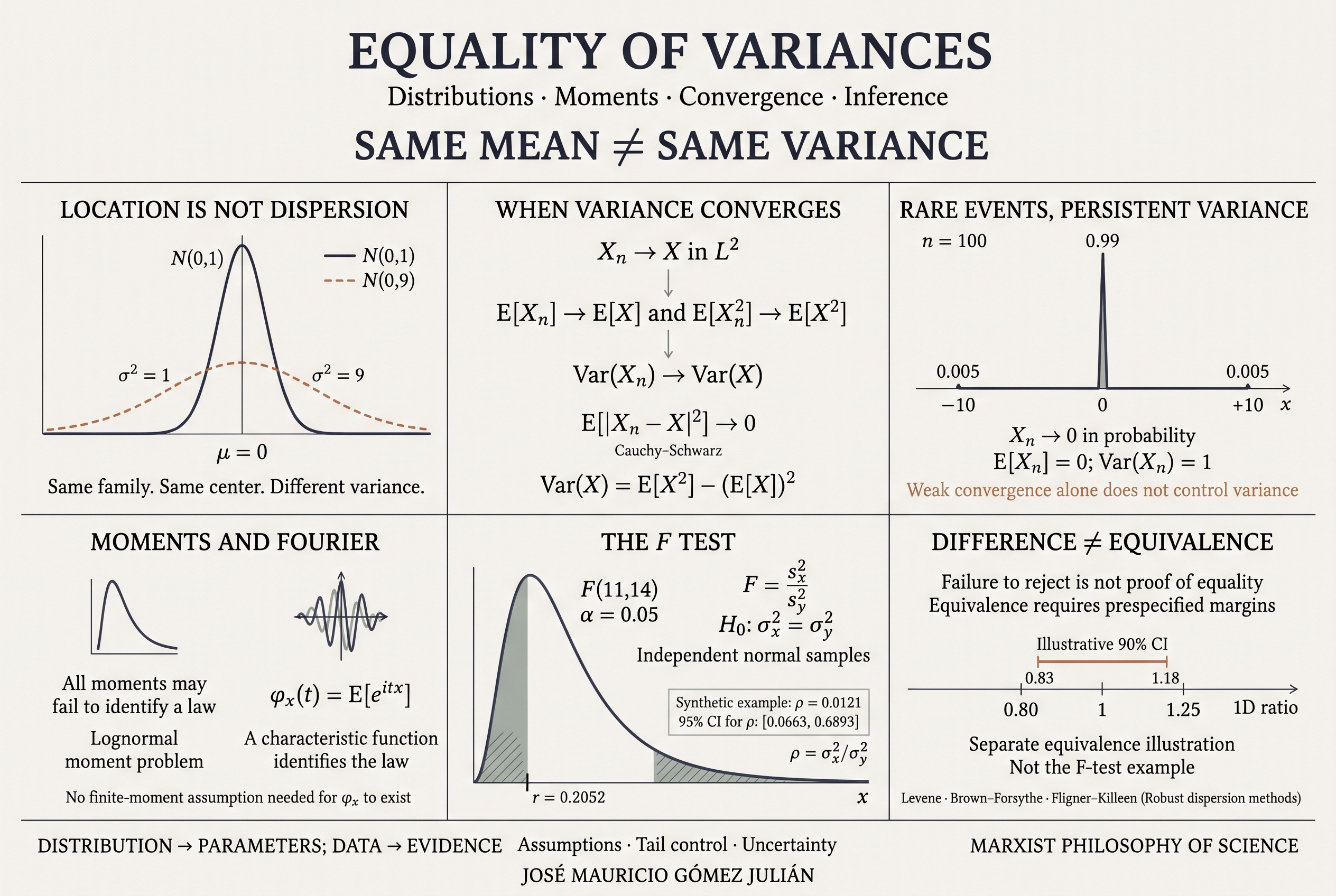
E[X] = E[Y] = 0; Var(X) = 1 ≠ 9 = Var(Y)
Our notation is N(μ, σ²): the second parameter is the variance.
A scale transformation changes variance itself: Var(a + bX) = b2Var(X). Preserving standardized shape therefore need not preserve dispersion in the original units.
The reverse implication also fails: a standard normal variable and a variable taking −1 and 1 with probability 1/2 both have mean zero and variance one, although one is continuous and the other discrete.
04Lʳ convergence and mean-square convergence
Convergence concerns a sequence of random variables and a limit, rather than an informal resemblance between two samples. For r ≥ 1, with the variables defined on the same probability space, Lr convergence means:
The case r = 1 is convergence in mean; r = 2 is mean-square convergence.
Convergence of E[Xn] to E[X] alone does not give L1 convergence: the expectation of a signed difference can conceal cancellations. L1 distance uses the absolute value. Likewise, a test of means does not measure the L2 distance between variables.
In L2, the norm ‖X‖2 = (E[|X|2])1/2 arises from the inner product E[XY]. This Hilbert-space structure explains the usefulness of quadratic tools; it does not turn every kind of convergence into L2 convergence. Probability theory also studies other Lr spaces. [1]
Proof: controlling the first and second moments
Cauchy–Schwarz, also applied to the constant random variable one, gives:
For the squares, factor the difference and apply Cauchy–Schwarz again:
≤ ‖Xn − X‖2 · ‖Xn + X‖2 → 0
The second norm is bounded because ‖Xₙ + X‖₂ ≤ ‖Xₙ − X‖₂ + 2‖X‖₂.
Finally, use Var(Xn) = E[Xn2] − E[Xn]2. The result is convergence to a limit, with no arbitrary residual constant.
05Why convergence in distribution is not enough
The chain L2 ⇒ convergence in probability ⇒ convergence in distribution is valid; the reverse implications fail in general. Convergence in distribution controls expectations of bounded continuous functions, whereas x2 is unbounded.
For each integer n ≥ 1, consider a variable whose mass increasingly concentrates at zero, while retaining rare and increasingly extreme events:
P(Xn = 0) = 1 − 1/n
The two extreme probabilities add to 1/n; all three probabilities add to one.
For any ε > 0 and sufficiently large n, P(|Xn| > ε) = 1/n → 0. Hence Xn → 0 in probability and in distribution. Nevertheless:
E[Xn2] = n · (1/n) = 1;
Var(Xn) = 1 ≠ 0 = Var(0)
Decreasing frequency and increasing magnitude of the extremes offset each other exactly.
This example even converges to zero in L1, since E[|Xn|] = 1/√n → 0, yet its variances still fail to converge to the variance of the limit.
A sufficient additional condition for convergence in distribution to yield convergence of the first two moments is uniform integrability of the squares:
This prevents a persistent share of the second moment from escaping into increasingly distant tails.
For example, supnE[|Xn|2+δ] < ∞ for some δ > 0 is sufficient for this control. Bounded second moments alone are insufficient, as the counterexample shows. [1]
06Existence of moments and determination of the distribution
Once a distribution is fixed, every existing moment has a definite value. A separate question is whether knowing all the moments uniquely identifies that distribution. This is the moment problem. Having finite moments of every order does not, by itself, solve it.
Distributions with finite support or support contained in a compact interval are determined by their moments. Countability of an infinite support alone is insufficient. General sufficient conditions include a moment-generating function finite on an open neighborhood of zero and Carleman’s criterion. These conditions also cover continuous distributions. [2]
An explicit example: a family sharing the lognormal moments
Let f0 be the standard lognormal density, meaning log(X) ∼ N(0,1). For −1 ≤ a ≤ 1, define:
The bracketed factor is nonnegative. The perturbation integrates to zero and preserves normalization.
For every integer k ≥ 0, substituting z = log x and using the normal transform gives:
= exp(k2/2 − 2π2) sin(2πk) = 0
The oscillation disappears in every integer moment, even though the densities change with a.
These distinct densities therefore have exactly the same moments E[Xk] = exp(k2/2). Comparing variances requires only the first two moments; identifying an entire distribution is a more demanding problem.
07Characteristic functions and the Fourier transform
A characteristic function provides a representation identifying the complete law of a real random variable. Its general definition uses the distribution as a measure, so it does not presume that a density exists:
When a density f exists, the integral becomes ∫ eⁱᵗˣ f(x) dx. The dF definition includes discrete and mixed laws.
It exists for every real t because |eitX| = 1. Two variables have the same law if and only if their characteristic functions agree for every t. This uniqueness does not require moments to exist. [3]
If E[X2] < ∞, derivatives at zero recover the relevant moments:
Var(X) = −φ″X(0) − (E[X])2
The whole function identifies the law; these two derivatives recover the mean and variance.
The exponent’s sign and the Fourier normalization factors depend on the chosen convention. Here we use eitx. Inversion theorems, under their respective conditions, recover a measure or density; they do not introduce a free constant justifying an arbitrary difference between variances.
Characteristic functions do not automatically make the moments of a sequence converge either. Pointwise convergence to a limiting characteristic function gives convergence in distribution, but passing to unbounded moments still requires additional tail control.
08From populations to samples: consistency
Let X1, …, Xn be independent and identically distributed observations from a population with finite second moment. The usual sample variance is:
= [n/(n − 1)]{[1/n]∑i=1nXi2 − X̄n2}
The n − 1 divisor makes this estimator unbiased under i.i.d. sampling; the second-line identity establishes consistency.
The strong law of large numbers, applied to X and X2, gives X̄n → E[X] and n−1∑Xi2 → E[X2] almost surely. Thus Sn2 → σX2 almost surely. A finite fourth moment is unnecessary for this consistency, although certain results about its asymptotic distribution may require it.
For two samples, as both sizes grow, the estimators converge to their respective parameters:
The limit is zero if the population variances agree. Equal sample sizes n = m are unnecessary.
If both samples are known to come from the same law, equality of the parameter is already part of that assumption. Their observed sample variances may still differ. If common origin is a conjecture, evidence must come from the data.
This asymptotic argument is not automatically an approach to the size of a finite population: sampling without replacement changes dependence and design. Nor does it justify ignoring temporal correlation, clusters, or paired measurements.
09The F test: assumptions, derivation, and interval
For two independent samples, each i.i.d. from a normal population with positive variance, define ρ = σX2/σY2. Equality means ρ = 1. The two-sided test contrasts H0: ρ = 1 against H1: ρ ≠ 1. [4]
[(m − 1)SY2]/σY2 ∼ χ2m−1
Normality yields these chi-squared distributions; independent samples make the two normalized numerators independent.
An F variable is a ratio of independent chi-squared variables, each divided by its degrees of freedom.
Under H0, the statistic F = SX2/SY2 follows this distribution without the factor ρ. Degrees of freedom identify the numerator and denominator order; they must not be inadvertently interchanged.
Let qu be the lower-tail quantile defined by P(Fn−1,m−1 ≤ qu) = u. At level α, reject when the observed ratio r lies outside [qα/2, q1−α/2]. This quantile convention agrees with R’s qf.
G is the F cumulative distribution function under H₀. This is the equal-tail two-sided version; computation uses the upper tail directly for numerical stability.
The interval comes from inverting the F/ρ pivot; inversion reverses the quantile order.
The ratio is dimensionless. An interval containing one is compatible with equality at the corresponding level, but does not prove it. If reduced variability is the target, the one-sided direction should be specified before examining results. Normality is a condition for this exact result; a nonsignificant normality test cannot certify it. [5]
10Robust alternatives and the scope of their hypotheses
The classical F test is sensitive to departures from normality. For skewed data or extreme observations, consider procedures that do not rely on the same normal-theory pivot. Robustness must always be related to the design and the target parameter.
| Procedure | Construction and interpretation |
|---|---|
| Levene | Uses ANOVA to compare absolute deviations from group means. |
| Brown–Forsythe | A median-centered Levene variant that reduces the influence of extreme observations. |
| Fligner–Killeen | Uses ranks and normal scores of median-centered absolute deviations. |
| Resampling methods | Require justified conditions; a naive permutation requires exchangeability, which equal variances alone do not imply. |
Brown–Forsythe constructs Zij = |Xij − mediani| and compares the means of Z across groups. Its calibration is approximate, unlike the exact normal-theory F test. When distributional shapes differ substantially, equal expected absolute deviations and equal variances are not generally equivalent. [6] [7]
For a common location–scale family, interpretation as a scale comparison is more direct. If variance does not exist, as for a Cauchy law, the target must change, for example to a quantile-based measure of dispersion, and that change must be stated.
If the substantive objective is to compare means, Welch’s test permits this without imposing equal variances. Mechanically choosing between Student and Welch after a preliminary variance test adds a selection step; the procedure should follow the design and inferential objective. [8]
11Non-rejection, power, and practical equivalence
A p-value greater than α means that the test supplies insufficient evidence to reject H0 at the chosen level. It is not the probability that H0 is true. An uninformative study may produce this result even when meaningful differences exist.
Power is defined against a specific alternative: π(ρ) = Pρ(reject H0). For the equal-tail two-sided F test, a positive alternative ratio ρ, and normal-theory assumptions:
+ 1 − G(q1−α/2/ρ)
The sample ratio has distribution ρF. Both quantiles and G use the design’s degrees of freedom.
| n per group | Power at ρ = 0.5 |
|---|---|
| 12 | 0.1885 |
| 30 | 0.4478 |
| 60 | 0.7517 |
| 120 | 0.9643 |
These are prospective calculations for a specified scenario, rather than estimates derived from the example’s p-value. The relevant difference and the sample sizes should be planned together; equal means cannot replace that work.
To establish practical equivalence, prespecify limits L and U representing tolerable differences, with 0 < L < 1 < U. The question becomes whether L < ρ < U:
H1eq: L < ρ < U
The equivalence null represents differences that are too large, rather than point equality.
With two one-sided tests at level α, declare equivalence only when both reject. Under the normal model, this is equivalent to the two-sided 1 − 2α confidence interval for ρ lying entirely within (L,U). At α = 0.05 this uses a 90% interval, rather than a 95% interval.
As a conceptual illustration, a 90% interval [0.83,1.18] would lie inside (0.80,1.25). These reciprocal margins express multiplicative tolerance; they are neither a universal recommendation nor results from the example below. The substantive problem must justify them.
12A fully reproducible numerical example
We use two synthetic samples generated from independent normal models X ∼ N(10,1) and Y ∼ N(10,4). Their population means agree by construction; their population variances differ. The vectors are fixed to six decimal places in the code, so the results do not depend on R’s random-number generator.
| Summary | Sample X | Sample Y |
|---|---|---|
| Sample size | 12 | 15 |
| Sample mean | 10.012313 | 9.320673 |
| Sample variance | 0.634224 | 3.090340 |
df = (11,14); p = 0.012080
CI95%(ρ) = [0.066318, 0.689321]
Decimal points match the code to make reproduction straightforward.
At level 0.05, equality is rejected within the normal model. The interval lies below one: the evidence favors a smaller variance for X than for Y. The point estimate is about 20.5% of Y’s variance, but the interval shows substantial uncertainty. The population ratio used in simulation is 1/4; individual sample ratios need not match it exactly.
As sensitivity analyses, Brown–Forsythe yields F = 7.973726 and p = 0.009182; Fligner–Killeen yields χ² ≈ 6.840015 and p ≈ 0.008914. Agreement here does not make their hypotheses identical or establish universal robustness. Choose the primary method before searching for the most favorable result.
13R code: computation, sensitivity, and diagnostics
The code below uses only base R functions. It reproduces the test, checks its formulas, computes the two sensitivity analyses, and applies the equivalence criterion using illustrative margins. Q–Q plots and a boxplot support inspection without becoming an automatic assumptions test. Inferential validity still depends on the design and model.
View complete code · copy and run in R or RStudio
# Igualdad de varianzas / Equality of variances
# Datos sinteticos fijos / Fixed synthetic data
# R base: stats + graphics; no external packages.
x <- c(9.867324, 10.005934, 9.230461, 10.707670,
       10.857477, 8.684811, 9.164998, 10.428310,
       9.504457, 10.836370, 11.206876, 9.653071)
y <- c(10.769160, 11.227355, 10.982203, 8.646258,
       7.303017, 7.526147, 11.072729, 7.522827,
       8.943126, 8.643210, 9.186375, 12.431695,
       7.238559, 7.421358, 10.896078)
stopifnot(all(is.finite(c(x, y))), var(x) > 0, var(y) > 0)

# Resumen / Summary
resumen <- data.frame(
  group = c("X", "Y"), n = c(length(x), length(y)),
  mean = c(mean(x), mean(y)), variance = c(var(x), var(y)))
print(resumen, digits = 8)

# F bilateral e IC / Two-sided F test and CI
alpha <- 0.05
nu1 <- length(x) - 1
nu2 <- length(y) - 1
r <- var(x) / var(y)
test_F <- var.test(x, y, ratio = 1, conf.level = 1 - alpha)
p_manual <- min(1, 2 * min(pf(r, nu1, nu2),
                         pf(r, nu1, nu2, lower.tail = FALSE)))
ci_manual <- c(r / qf(1 - alpha/2, nu1, nu2),
               r / qf(alpha/2, nu1, nu2))
stopifnot(abs(unname(test_F$statistic) - r) < 1e-10,
          abs(test_F$p.value - p_manual) < 1e-10,
          max(abs(as.numeric(test_F$conf.int) - ci_manual)) < 1e-10)
print(test_F)

# Brown-Forsythe: ANOVA de desviaciones absolutas / of absolute deviations
datos <- data.frame(
  value = c(x, y),
  group = factor(c(rep("X", length(x)), rep("Y", length(y)))))
datos$absdev <- abs(datos$value -
                   ave(datos$value, datos$group, FUN = median))
bf <- anova(lm(absdev ~ group, data = datos))
print(bf)
fk <- fligner.test(value ~ group, data = datos)
print(fk)

# Equivalencia / Equivalence: illustrative margins, not universal
L <- 0.80
U <- 1.25
ci90 <- c(r / qf(1 - alpha, nu1, nu2),
          r / qf(alpha, nu1, nu2))
p_lower <- pf(r / L, nu1, nu2, lower.tail = FALSE)
p_upper <- pf(r / U, nu1, nu2)
p_tost <- max(p_lower, p_upper)
equivalent <- all(ci90 > L & ci90 < U)
stopifnot(identical(equivalent, p_tost < alpha))
print(list(CI90 = ci90, margins = c(L, U),
           p_TOST = p_tost, equivalent = equivalent))

# Potencia prospectiva / Prospective power under independent normal samples
power_F <- function(n1, n2, rho, alpha = 0.05) {
  stopifnot(n1 >= 2, n2 >= 2, n1 == as.integer(n1),
            n2 == as.integer(n2), rho > 0, alpha > 0, alpha < 1)
  df1 <- n1 - 1
  df2 <- n2 - 1
  q <- qf(c(alpha/2, 1 - alpha/2), df1, df2)
  pf(q[1]/rho, df1, df2) +
    pf(q[2]/rho, df1, df2, lower.tail = FALSE)
}
sizes <- c(12, 30, 60, 120)
print(data.frame(n_per_group = sizes,
  power_rho_0.5 = vapply(sizes, function(n) power_F(n, n, 0.5), numeric(1))))
stopifnot(abs(power_F(12, 15, 1) - alpha) < 1e-10)

# Diagnosticos / Diagnostics; no automatic normality-test gate
op <- par(mfrow = c(1, 3))
boxplot(value ~ group, data = datos, col = "#fffdf7",
        border = "#8b4513", xlab = "Group", ylab = "Value")
qqnorm(x, main = "X: normal Q-Q"); qqline(x, col = "#8b4513")
qqnorm(y, main = "Y: normal Q-Q"); qqline(y, col = "#8b4513")
par(op)
sessionInfo()
The manual calculation and var.test should agree numerically. This example does not establish equivalence within (0.80,1.25). Brown–Forsythe is implemented through ANOVA of absolute deviations, and fligner.test follows R’s documented procedure. [5] [7]
14Homogeneity, the structure of the phenomenon, and abstraction
Statistical homogeneity must be specified: equal variances, equal distributions, and exchangeability are distinct properties. Their relevance depends on the unit of analysis, measurement scale, selection process, and relationships among observations.
A population mixing subgroups shows how the phenomenon’s structure enters total variability. If G identifies the subgroup and X has finite second moment, the law of total variance states:
Total dispersion includes variability within groups and variability between their means.
Two populations can have identical within-subgroup variances yet different total variances when the separation of subgroup means or the mixture composition changes. For example, if each subgroup has variance one, their means are −a and a, and each has weight 1/2, total variance is 1 + a2. Structural heterogeneity thus enters an explicit mathematical result.
From a materialist perspective, statistical abstraction selects relationships within the phenomenon and must justify that selection. A theorem establishes what follows from assumptions; research determines whether those assumptions adequately represent the material process. Larger samples can reduce uncertainty without correcting an ill-defined population, omitted dependence, or a misspecified mixture.
15Conclusions: conditions before shortcuts
Equal variances can follow from a known distributional identity or be investigated through appropriate estimation and testing. Equal means, standardized shape, and sample size cannot replace that justification.
L2 convergence permits passage to the limiting variance; convergence in distribution needs additional conditions controlling second moments. Characteristic functions identify complete laws, whereas determination by moments requires its own conditions.
With finite data, the variance ratio and its confidence interval explain the size and uncertainty of dispersion differences. Power evaluates the design’s ability to detect differences; equivalence requires prior substantive margins. Each conclusion must match its target, model, and actual supporting evidence.
References and further reading
- MIT OpenCourseWare. Fundamentals of Probability (2018), lectures 16–19. Read source.
- Lin, G. D. (2017). Recent developments on the moment problem. Journal of Statistical Distributions and Applications, 4, 5. DOI: 10.1186/s40488-017-0059-2. Read source.
- Duke University. The Probability Workbook: Characteristic functions (aka Fourier Transforms). Read source.
- NIST/SEMATECH. e-Handbook of Statistical Methods, §1.3.5.9, F-Test for Equality of Two Variances. Read source.
- R Core Team. stats: var.test — F Test to Compare Two Variances. Read source.
- NIST/SEMATECH. e-Handbook of Statistical Methods, §1.3.5.10, Levene Test for Equality of Variances. Read source.
- R Core Team. stats: fligner.test — Fligner-Killeen Test of Homogeneity of Variances. Read source.
- R Core Team. stats: t.test — Student’s t-Test (Welch procedure when var.equal = FALSE). Read source.
Leave a Comment/Deja un Comentario