
Marxist Philosophy of Science · Statistics and political economy
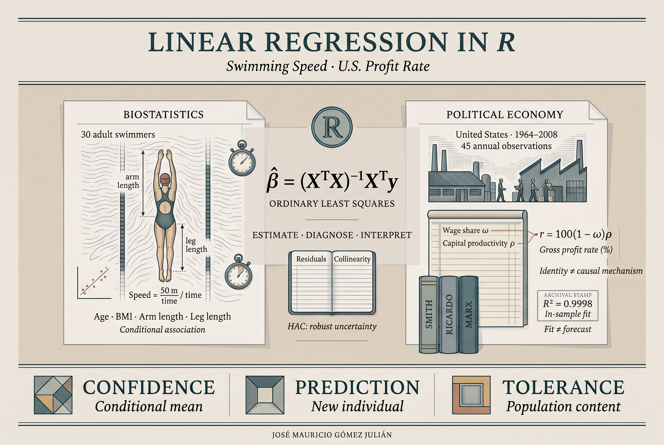
The Classical Linear Regression Model in R
Foundations, calculation, and interpretation: from swimming speed to the rate of profit
Originally published: December 1, 2021
Revised and expanded: November 4, 2026
01One scientific question, two fields of application
Regression connects a question about the world with a mathematical representation of its regularities. Its scientific value depends on measurement quality, research design, the assumptions linking data to the model, and the historical and material interpretation of the phenomenon. Numerical fit is part of that process.
This article examines the classical linear regression model through two applications: adult swimming speed and the gross rate of profit in the United States during 1964–2008. The first develops matrix calculations, standardisation, the decomposition of variability, and uncertainty. The second also requires examining how variables are constructed from accounting data, temporal dependence, and the relationships between distribution, productivity, and profitability.
The exposition combines algebra, geometry, probability, R programming, and political economy. Equations are accompanied by interpretations, tables identify their provenance, and the final laboratory includes all the synthetic data needed to run it.
02Population, sample, and notation
Let Y be a response variable and X1, …, Xk the predictors. For observation i, the additive model with an intercept is:
β₀ is the intercept; βⱼ is a population slope; uᵢ captures the difference between the response and the part represented by the model.
We use n for the number of observations and p = k + 1 for the number of coefficients, including the intercept. The design matrix X has n rows and p columns; its first column contains ones. Vector β has p components, and y contains the observed responses.
A random variable, its observed realisation, a population parameter, and its estimator are distinct objects. β̂ is an estimator before a sample is observed and a numerical estimate once the data are fixed. Similarly, ui is an unobserved population error; ei = yi − ŷi is a calculated residual.
Expectation is a probabilistic operator; the arithmetic mean is a function of the data that can estimate an expectation under appropriate conditions. Distinguishing them does not sever their relationship. Nor should a marginal distribution automatically be equated with a Bayesian prior: the former integrates out conditioning variables, whereas the latter represents uncertainty about parameters before updating.
03What makes the model linear
Linearity refers to the coefficients. A model containing age and age squared is still linear in its parameters. So is a model containing an interaction between the wage share and capital productivity.
In this specification, the slope with respect to X is β1 + β3Z. Adding an interaction therefore changes the meaning of the individual slopes. Coefficient β1 describes the statistical effect of X when Z equals zero, subject to the model’s interpretation.
Transforming the response also changes the quantity being estimated. When log speed is modelled, exponentiating the predicted mean of log speed does not generally recover mean speed: back-transformation requires considering the error distribution. Likewise, modelling travel time and then transforming through 50/time is not equivalent to directly fitting mean speed.
04Least squares: optimisation and projection
Ordinary least squares (OLS) chooses the coefficients that minimise the sum of squared residuals. Squared loss penalises large errors particularly strongly.
Differentiating with respect to b and setting the derivative equal to zero yields the normal equations XTXb = XTy. If the columns of X are linearly independent, the solution is unique:
Geometrically, ŷ is the orthogonal projection of y onto the space spanned by the columns of X. Residuals are orthogonal to that space: XTe = 0. With an intercept, residuals sum to zero apart from rounding error.
This orthogonality of residuals to the design columns does not require predictors to be mutually orthogonal. The former is an algebraic property of the fit; the latter would be an additional property of the design.
X <- model.matrix(~ edad + imc + pierna + brazo, data = bio)
y <- bio$veloc
# Teaching expression; requires full rank and good conditioning.
beta_ecuaciones <- solve(crossprod(X), crossprod(X, y))
# Preferred for numerical computation: QR decomposition.
beta_qr <- qr.coef(qr(X), y)
m_bio <- lm(veloc ~ edad + imc + pierna + brazo, data = bio)
all.equal(unname(beta_qr), unname(coef(m_bio)))
Inverting XTX is useful for deriving formulas. In computation, forming this product can worsen numerical conditioning; lm() uses QR. An exact mathematical identity and a floating-point operation involve different levels of representation: small discrepancies are assessed using explicit numerical tolerances.
05What each assumption guarantees
| Condition | What it supports | What it does not establish |
|---|---|---|
| Full column rank of X | Unique identification of OLS coefficients. | Stochastic independence between predictors. |
| E(u | X) = 0 | Conditional unbiasedness of OLS, subject to the relevant existence conditions. | Causality simply because a regression has been fitted. |
| Var(u | X) = σ²I | Classical covariance and OLS efficiency among linear unbiased estimators. | Normality of errors. |
| Conditional normality of u | Exact t and F distributions in a correctly specified classical model. | Marginal normality of every predictor or of Y. |
| Moment and weak-dependence conditions | Relevant laws of large numbers and asymptotic approximations. | That 30 or 45 observations automatically constitute a large sample. |
| Causal design and substantive identification | Causal interpretation under the design-specific assumptions. | That a small p-value replaces identification. |
Normality is unnecessary for computing OLS or for the Gauss–Markov theorem. Heteroskedasticity does not, by itself, bias the coefficients if exogeneity holds, but it invalidates the conventional covariance formula. Consistency requires additional conditions on the generating process, its moments, and its dependence.
Linear independence means that no column is an exact linear combination of the others. Stochastic independence concerns the factorisation of joint distributions. Orthogonality means a zero inner product. Zero correlation is another property and does not, in general, imply stochastic independence.
06The swimming case: measurement and target population
The application considers regular swimming-team members completing 50 metres. The documented tables contain 30 observations, with ages ranging from 18 to 51. Describing the sample as people aged 18 or older is more precise than describing everyone as strictly older than 18.
| Variable | Definition and unit | Interpretive caution |
|---|---|---|
| veloc | Swimming speed, in metres per second. | A higher value means faster swimming; using time reverses the direction. |
| edad | Age in completed years. | The cross-sectional coefficient compares people; it does not automatically measure individual ageing. |
| sexo | Documented coding: 0 women, 1 men. | Document the coding rather than assigning it a single biological explanation. |
| imc | Weight in kg divided by squared height in metres: BMI. | Not a direct measure of body composition. |
| pierna | Mean length of both legs, in cm. | May share variation with arm length and other body measurements. |
| brazo | Mean length of both arms, in cm. | Its adjusted association depends on the predictors included. |
The target population is shaped by recruitment: regular team membership does not represent the entire adult population. Training, technique, health, experience, and selection into participation can influence both observed characteristics and performance.
Omitting sexo from some models does not establish identical mean speed across its categories. Such a model describes a relationship without explicit adjustment for that variable. Inclusion or exclusion should be discussed in terms of the question, design, and sample size, avoiding decisions based solely on marginal correlations.
07Graphical exploration and correlations
Scatterplots help examine approximate linearity, extreme observations, sparsely populated regions, and possible group differences. A fitted line summarises a trend; a smoother helps explore curvature. Plot bands must be interpreted according to the procedure producing them: they do not automatically represent a concentration region for errors.
# With bio defined in the final laboratory:
vars <- c("veloc", "edad", "imc", "pierna", "brazo")
pairs(bio[vars], pch = 19, col = "#8b4513")
round(cor(bio[vars]), 3)
# Optional; the corresponding packages are required.
# lattice::xyplot(veloc ~ edad, data = bio, type = c("p", "r"))
# car::scatterplot(veloc ~ edad, data = bio)
# car::scatterplotMatrix(~ veloc + edad + imc + pierna + brazo, data = bio)
In xyplot(), type=c("p","r") requests points and a regression line. It is a plotting argument, not an instruction to change an object’s storage type. Trellis names a system of conditioning plots; using the lattice package does not imply constructing an algebraic lattice in the sense of order theory.
The documented correlations with speed are approximately −0.65 for age, −0.01 for BMI, 0.21 for leg length, and 0.29 for arm length. These describe bivariate sample associations. A small marginal correlation does not establish irrelevance after adjusting for other variables, and a strong correlation does not identify a causal effect.
Pearson’s coefficient is covariance divided by the product of standard deviations. It is unitless and describes linear association. It should be examined alongside the plot: outliers, mixed groups, or curvature can make its scalar summary misleading.
08Comparable specifications and modelling decisions
| Stable name | Specification | Question |
|---|---|---|
| m_dos | veloc ~ edad + brazo | Associations adjusted for age and arm length. |
| m_bio | veloc ~ edad + imc + pierna + brazo | Conditional contributions of four characteristics. |
| m_sin_edad | veloc ~ imc + pierna + brazo | What changes when age is omitted. |
| m_mm | veloc ~ edad + imc + pierna + brazomm | Invariance of fitted values after a unit change. |
| m_edad | veloc ~ edad | What age describes by itself. |
| m_nulo | veloc ~ 1 | Reference based on a common mean. |
Model comparisons require retaining the same observations. If each fit removes different rows because of missing values, its sums of squares and information criteria cease to be directly comparable. The treatment of missingness must be defined and documented before comparison.
Dropping leg length because it is highly correlated with arm length may reduce instability, but it also changes the question and can introduce omitted-variable bias if a necessary variable is removed. Examining rank, variance inflation, substantive knowledge, and stability provides a fuller assessment.
m_dos <- lm(veloc ~ edad + brazo, data = bio)
m_bio <- lm(veloc ~ edad + imc + pierna + brazo, data = bio)
m_sin_edad <- lm(veloc ~ imc + pierna + brazo, data = bio)
m_edad <- lm(veloc ~ edad, data = bio)
m_nulo <- lm(veloc ~ 1, data = bio)
stopifnot(nobs(m_bio) == nobs(m_edad), nobs(m_bio) == nobs(m_sin_edad))09Interpreting slopes and point predictions
The documented age-and-arm-length specification yields approximately:
Comparing two people ten years apart in age, holding arm length fixed, is associated with a difference of −0.1816942 m/s in estimated mean speed. A five-centimetre difference in arm length, at a fixed age, is associated with +0.107098 m/s. These are conditional model comparisons; they do not necessarily describe how the same person would change after ten years or after an intervention.
For age 24 and arm length 71 cm, the documented prediction is 1.376928 m/s. For age 34 with the same arm length, it is 1.195234 m/s. Keep the full coefficient precision during calculation and round for presentation: 1.38 and 1.20 m/s.
# x0 builds a new predictor combination; it does not select rows.
x0 <- c(1, 24, 71)
# For the model fitted to the data currently in use:
drop(x0 %*% coef(m_dos))
predict(m_dos, newdata = data.frame(edad = 24, brazo = 71))
The first component of x0 is the one multiplying the intercept. This model’s intercept corresponds to age zero and arm length zero, a scenario without an applied interpretation in the adult sample. Its algebraic role does not require assigning it a real biological state.
10Units and standardised coefficients
If a length is converted from centimetres to millimetres, its values are multiplied by ten and its slope is divided by ten. Predictions, residuals, and the residual sum of squares remain unchanged apart from rounding. Changing units adds no explanatory capacity.
The fully standardised slope expresses differences in standard deviations of Y per one standard deviation of Xⱼ, holding the other variables fixed.
In the documented four-predictor specification, standardised slopes are approximately −0.76 for age, 0.20 for BMI, −0.07 for leg length, and 0.50 for arm length. The comparison refers to that sample and that set of controls. Standard deviations incorporate features of the sample distribution, so the ordering of magnitudes is not a universal causal ranking.
Rₓₓ is the correlation matrix of centred and scaled predictors; rₓᵧ contains their correlations with the response. Rₓₓ must be invertible.
In simple regression with an intercept, the fully standardised slope equals Pearson’s correlation. In multiple regression, it equals each predictor’s bivariate correlation if the standardised predictors are mutually orthogonal. Orthogonality can occur with continuous variables or with factors under suitable designs.
vars <- c("veloc", "edad", "imc", "pierna", "brazo")
bio_z <- as.data.frame(scale(bio[vars]))
m_z <- lm(veloc ~ edad + imc + pierna + brazo, data = bio_z)
beta_est <- coef(m_bio)[-1] * sapply(bio[vars[-1]], sd) / sd(bio$veloc)
all.equal(unname(beta_est), unname(coef(m_z)[-1]))11Sums of squares and degrees of freedom
For OLS with an intercept, total variability around the mean decomposes into variability explained by the fit and residual variability:
We use SST for the total sum of squares, SSR for the regression sum of squares, and SSE for the residual error sum of squares. Some sources use different abbreviations, so each name should always be accompanied by its defining formula.
s² is the residual mean square and estimates σ² under the classical assumptions. MSR is the regression mean square for the set of slopes. Degrees of freedom are not identical for all terms: they depend on rank and the number of restrictions.
The residual projection has dimension n − p. Estimating a mean imposes one restriction on residuals and leaves n − 1 degrees of freedom. More generally, degrees of freedom are explained by linear restrictions and rank, without needing to derive them from a physical principle of least action.
| Documented model | SSE | s² | R² | Adjusted R² |
|---|---|---|---|---|
| Four predictors | 0.64517 | 0.0258068 | 0.62707 | 0.56740 |
| Without age | 1.56336 | 0.0601292 | 0.09633 | −0.00794 |
| Age only | 0.99021 | 0.0353646 | 0.42763 | 0.40718 |
The four-predictor model captures approximately 62.7% of sample variability; age alone captures 42.8%. Adding predictors to nested models on the same rows never reduces ordinary R². This mechanical property explains the need to consider complexity and validation.
A negative adjusted R² indicates that, under this penalty, the specification performs worse than a common-mean reference. Equality of two R² values after rounding does not establish the absence of overfitting.
An estimator’s quadratic risk is a different object: MSE(θ̂) = Var(θ̂) + Bias(θ̂)². It should not simply be identified with the residual mean square. In predictive evaluation, RMSE usually uses the average squared error on test observations; its denominator serves a different purpose from estimating σ² using n − p.
12Covariance, standard errors, and coefficient intervals
Under Var(u | X) = σ²I, slope uncertainty depends on residual variability and the geometry of the design.
The diagonal contains estimated coefficient variances. Their square roots are standard errors. Off-diagonal elements are covariances between estimators and matter when calculating uncertainty for combinations of coefficients.
| Term | Estimate | Standard error | Documented 95% CI |
|---|---|---|---|
| Intercept | −0.135422 | 0.602032 | [−1.3753, 1.1045] |
| Age (edad) | −0.019172 | 0.003214 | [−0.0258, −0.0126] |
| BMI (imc) | 0.015532 | 0.010023 | [−0.0051, 0.0362] |
| Leg length (pierna) | −0.002599 | 0.009907 | [−0.0230, 0.0178] |
| Arm length (brazo) | 0.026262 | 0.012982 | [−0.0005, 0.0530] |
For a five-year difference, holding the other characteristics fixed, the mean-difference interval is obtained by multiplying both endpoints of the age interval by five: approximately [−0.129, −0.063] m/s. Multiplying by a negative constant would also require reordering the endpoints.
The precision of slopes measured in different units cannot be compared using the absolute widths of their intervals. An interval excluding zero concerns the corresponding two-sided test; it does not establish that the coefficient has the greatest scientific importance.
13Conditional mean and new observation: two uncertainties
For a combination of characteristics x0, the predicted mean is x0Tβ̂. Its estimated variance is a quadratic form:
A new observation adds its own individual variation. Under normality, homoskedasticity, and independence of the new error from the sample:
The additional s² term explains why the individual interval is wider. For age 22, BMI 20 kg/m², leg length 100 cm, and arm length 70 cm, the documented outputs are:
| Quantity | Estimate or interval | Interpretation |
|---|---|---|
| Predicted mean | 1.33 m/s | Estimated conditional mean speed. |
| 95% CI for the mean | [1.22, 1.45] m/s | Uncertainty about the conditional mean. |
| 95% individual PI | [0.98, 1.68] m/s | Predictive coverage for a new observation under the model. |
nuevo <- data.frame(edad = 22, imc = 20, pierna = 100, brazo = 70)
predict(m_bio, nuevo, interval = "confidence", level = .95)
predict(m_bio, nuevo, interval = "prediction", level = .95)
In a frequentist interpretation, the confidence level describes procedural coverage under repeated sampling. It does not mean that 95% of people fall within the interval for the mean, nor does it constitute causal evidence. The specific numbers above belong to the documented study; running the synthetic laboratory will produce different intervals.
14Tolerance and Bayesian inference: a different question
A tolerance interval seeks to cover at least a proportion P of a distribution with confidence 1 − α. Content and confidence are separate controls. A prediction interval for one future observation does not automatically provide the same guarantee about a population fraction.
This expression states the frequentist content guarantee for a two-sided tolerance interval.
For a marginal normal distribution, the usual form is ȳ ± ktols. The tolerance factor depends on sample size, confidence, content, and procedure. An equal-tailed interval additionally controls how the excluded content is distributed between the two tails.
# Requires tolerance; synthetic marginal normal example.
# Not a conditional interval from the swimming model.
set.seed(20261106)
y_normal_demo <- rnorm(60, mean = 1.4, sd = .16)
# tolerance::normtol.int(y_normal_demo, alpha = .05, P = .95,
#                        side = 2, method = "HE")
Conditional regression tolerance requires a procedure incorporating covariates and their uncertainty. Applying a marginal procedure to all swimming speeds answers a different question.
A conjugate Bayesian normal formulation can specify μ | σ² ∼ N(μ₀, σ²/n₀), together with a scaled inverse-chi-squared distribution for σ² with parameters m₀ and s₀². Here μ₀ is a prior location; n₀ controls relative precision for μ; m₀ and s₀² govern prior uncertainty about σ². Neither n₀ nor m₀ is another observed mean or variance.
A normal likelihood and a prior distribution are distinct components. An approximately normal response histogram does not determine a prior over its parameters. Hyperparameters require external information, an explicit construction rule, or sensitivity analysis. In bayesnormtol.int(), one must also distinguish side=1, which produces one-sided limits, from side=2, which specifies a two-sided procedure.
Arbitrary moment matching does not justify a prior. Convergence in distribution alone does not ensure convergence of moments: additional conditions, such as appropriate uniform integrability, are required. Every probability distribution has a characteristic function, even when its mean or variance is not finite. The normal distribution has all its moments, but the existence of a characteristic function is not proof that all moments exist.
15Distributions, Q–Q, P–P, and normality tests
A Q–Q plot compares observed quantiles with quantiles of a reference distribution. A P–P plot compares cumulative probabilities. The former often makes tail discrepancies more visible; the latter provides another view of distributional fit.
In normal regression, the assumption concerns conditional errors. The marginal response may be skewed because it mixes groups or covariate values even when conditional errors are normal. Begin with residuals versus fitted values, residuals versus predictors, and a residual Q–Q plot.
par(mfrow = c(2, 2))
plot(m_bio)
par(mfrow = c(1, 1))
shapiro.test(residuals(m_bio))
# A test on fitted residuals is interpreted as exploratory diagnostics;
# residuals share restrictions and are not an iid sample of errors.
The documented Shapiro–Wilk output for the swimming response gives p = 0.3454. This does not reject marginal normality at 5%, but neither establishes normality nor verifies all regression assumptions.
A one-sample Kolmogorov–Smirnov test compares data with a fully specified distribution function. Its usual calibration does not apply when parameters are estimated from the same sample. Comparing the data with simulated normal observations having a different location and scale tests equality of distributions, rather than providing a general normal-shape diagnostic. A Lilliefors procedure or a properly designed simulation calibration addresses different issues and must be identified explicitly.
Fitting normal, lognormal, and gamma distributions by maximum likelihood allows comparison of candidate marginal models on the same response and sample. A lower AIC or BIC expresses a relative preference within that set, not a proof of truth. Moreover, a suitable marginal family does not by itself determine a regression’s conditional family.
ℓ is the maximised log-likelihood, and d counts the parameters estimated for that probabilistic model. Comparison requires a compatible likelihood basis.
With small datasets, considering corrected AIC may be appropriate if the formula matches the model family. Comparisons involving transformed responses must account for the transformation Jacobian; likelihood values defined on incompatible scales should not be compared directly.
16Marginal effects and sequential sums of squares
In an additive linear model, the partial derivative of the mean with respect to a continuous predictor is its slope:
Without interactions or transformations, the marginal effect is constant: the average marginal effect, the marginal effect at the means, and effects at representative values coincide. For a binary variable, calculate a discrete difference between predictions. None of these operations establishes causality without additional identification.
The reduction in the residual sum of squares when a variable is introduced is a different quantity. In anova(m_bio), terms are added in formula order. Their contributions depend on what came before; reordering terms does not change the slopes of the complete additive model.
| Documented quantity for leg length | Value | Comparison |
|---|---|---|
| Sequential sum of squares after age and BMI | 0.21680 | Add leg length before including arm length. |
| p-value of that ANOVA row | 0.007697 | Sequential test using the complete model’s residual mean square. |
| Adjusted p-value for leg length in summary() | 0.7952 | Leg-length coefficient conditional also on arm length. |
| Additional sum of squares after arm length, without other controls | 0.01660077 | Compare veloc ~ brazo with veloc ~ brazo + pierna. |
The difference between 0.007697 and 0.7952 is not a contradiction: the set of conditioning variables changes. The sequential test attributes to leg length variation it may share with arm length. To assess its contribution after all other terms, compare the complete model with one omitting only leg length, or use the equivalent t test for that single coefficient.
17t and F tests: explicit hypotheses and manual calculation
The p-value is the probability, under the null hypothesis and assumed model, of a test statistic at least as extreme as the observed one in the direction specified by the alternative. It is not the probability that the null is true, that the result is due to chance, or a general measure of a study’s reliability or importance.
For two nested models, reduced R and complete C, fitted on the same rows, let q = pC − pR be the number of restrictions. The classical statistic is:
Under the null hypothesis and spherical normal errors, it follows an F distribution with q and n − pC degrees of freedom. Large values provide evidence against the restrictions. Reject at level α if the p-value is below α, with the threshold set before examining results.
| Documented test | Null hypothesis | Approximate F | Approximate p-value |
|---|---|---|---|
| Four predictors versus age | β_BMI = β_leg = β_arm = 0 | 4.4567; df (3,25) | 0.012205 |
| Add age to the other three | β_age = 0 | 35.5794; df (1,25) | 0.000003153 |
| Four predictors versus intercept | All four slopes are zero | 10.5092; df (4,25) | 0.00003906 |
The first test indicates that the three additional variables, considered jointly, add information relative to the age-only model under classical assumptions. It does not establish that each is individually significant. Joint significance can coexist with inconclusive individual tests when predictors are correlated.
The equality concerns the same restriction, the same covariance estimator, and the equivalent two-sided t test. It does not equate every F test with every t test. Under the same procedure, a two-sided interval and the test at the corresponding level agree on excluding or including the null value.
anova(m_edad, m_bio)
anova(m_sin_edad, m_bio)
anova(m_nulo, m_bio)
# Upper tail, more stable than calculating 1 - pf(...):
F_doc <- ((.99021 - .64517) / 3) / (.64517 / 25)
pf(F_doc, df1 = 3, df2 = 25, lower.tail = FALSE)18Diagnostics: form, leverage, and influence
Residual analysis looks for patterns incompatible with the specification: curvature, fan-shaped dispersion, clusters, and dependence. A single plot neither verifies exogeneity nor removes the need to examine the design.
The leverage of observation i is diagonal element hii of the projection matrix. It summarises how unusual its predictor combination is relative to the design. A large residual describes response discrepancy. Influence measures how much a fit changes when observations are perturbed. These concepts are related but distinct.
Cook’s distance combines residual size and leverage. Thresholds such as 4/n or multiples of the mean are investigative guides. Measurement quality, context, and sensitivity of conclusions should be examined, without automatically deleting observations that reflect real episodes.
diagnostico <- data.frame(
  fila = seq_len(nobs(m_bio)),
  residuo = residuals(m_bio),
  residuo_studentizado = rstudent(m_bio),
  leverage = hatvalues(m_bio),
  Cook = cooks.distance(m_bio)
)
diagnostico[order(diagnostico$Cook, decreasing = TRUE), ]
An HC3 standard error helps assess inferential sensitivity to heteroskedasticity in a cross-sectional sample under appropriate conditions. It does not correct omitted variables, measurement error, dependence between swimmers, or sample selection.
19The rate of profit as a political-economy problem
Profitability connects investment decisions, competition, distribution, and capital reproduction. Studying it requires defining the surplus being measured, the capital used as denominator, its valuation, and the statistic’s institutional coverage.
Smith, Ricardo, and Marx give profits a central place, while offering different explanations of their movements and mediations. In Marx, surplus-value production, competition, the transformation of values into prices, and the formation of a general rate of profit belong to related levels of analysis. An aggregate national-accounts rate is a specific operationalisation; identifying it directly with a theoretical category requires an argument.
The Cambridge controversies over heterogeneous capital and reswitching challenge particular parables of substitution and aggregate marginal productivity. Their results should be presented within their formal scope: they do not, by themselves, empirically validate any alternative econometric specification.
Research on relationships between labour values and prices, and research on the determinants of profitability, share categories and sources but test different questions. A value–price correlation does not substitute for identifying the temporal mechanisms of a profit rate.
The exercise considered here uses 45 annual United States observations from 1964 to 2008 and attributes the data to the Extended Penn World Tables compiled by Marquetti and Foley. The time span allows historical trajectories to be examined, although the number of years does not by itself guarantee accurate asymptotic approximations.
20Define the variables before estimation
| Column | Interpretation to document | Required check |
|---|---|---|
| Mean_Gross_Profit | Gross rate of profit, expressed as a percentage. | Define surplus, denominator, and the difference between gross and net. |
| K_Productivity | Average capital productivity: output/capital. | Verify prices, coverage, and stock valuation. |
| L_Productivity | Average labour productivity: output per employed person. | Distinguish employment from hours and document the treatment of self-employment. |
| Mean_w_share | Labour compensation as a share of output. | Specify adjustments and consistency between numerator and denominator. |
| Mean_w | Average real wage or compensation per worker. | Confirm whether the column is a per-worker average; do not call it the total wage bill. |
| RealGDP | Aggregate real output. | Document currency, base year, purchasing power parity, and data vintage. |
| K_Net_Stock | Standardised net fixed capital stock. | Distinguish stock from flow, current valuation, and constant prices. |
| DepreciationRate | Depreciation rate. | Check whether the unit is a proportion or percentage. |
| Year | Calendar year. | Chronological order, no duplicates, and continuity of observations. |
Average capital productivity is not marginal capital productivity. The wage share is not the average wage, and the average wage is not the aggregate wage bill. Their changes can diverge: rising real remuneration can coexist with a falling wage share if productivity grows faster.
National accounts incorporate conventions and estimates. Their constructed character does not make them arbitrary: it means comparability, adjustments, and the relationship between statistical and theoretical categories are part of the investigation. Changing database editions can alter the series; replication requires identifying the exact edition.
21Accounting identities and shared relationships
Let Q be output, W labour compensation, K the capital stock, and N employment, defined consistently. Then:
If gross surplus is defined as Q − W, the gross rate of profit satisfies:
This construction of the gross rate appears explicitly in studies using EPWT 4.0. It must be checked against the exercise’s columns before concluding that it holds exactly: coverage, price, source, or rounding adjustments can change its numerical agreement. A net rate must incorporate depreciation consistently, using compatible units.
When these identities hold, regressing profitability on the wage share and capital productivity uses components of the response itself. A strong association may follow from that construction. Its economic content also concerns how the components evolve and why; the identity alone does not determine their causal mechanisms.
# Apply to empirical data only after confirming the definitions.
identidad_r <- with(eco, 100 * (1 - Mean_w_share) * K_Productivity)
identidad_w <- with(eco, Mean_w_share * L_Productivity)
max(abs(eco$Mean_Gross_Profit - identidad_r))
max(abs(eco$Mean_w - identidad_w))
The profitability identity is multiplicative in ω and ρ. Written as a regression, it contains an interaction:
An additive regression can approximate it very closely over a limited range without its four slopes representing four independent mechanisms. Moreover, w = ωx generates nonlinear functional dependence between predictors. This need not be perfect linear collinearity, but it restricts economically possible combinations.
Consequently, the partial derivative of a fit that holds the average wage and wage share fixed while changing labour productivity may describe a combination incompatible with these identities. A ceteris paribus interpretation must respect the set of admissible states.
22The economic model and the meaning of its fit
The documented four-predictor specification is:
| Documented result | Value | Appropriate reading |
|---|---|---|
| Observations | 45 years | A historical series; years are not exchangeable by default. |
| Estimated coefficients | 5, including the intercept | 40 residual degrees of freedom. |
| R² and adjusted R² | Both 0.9998 after rounding | Exceptionally high in-sample fit; investigate identities and validation. |
| Residual standard error | 0.0439 | In response units; if percentages are used, percentage points. |
| Intercept | Approximately 71.532 | Prediction at zero-valued predictors; potentially extreme extrapolation. |
A significant intercept does not demonstrate autonomous profitability independent of economic processes or identify omitted political factors. A constant can absorb the level of a local approximation and lack substantive meaning when the origin is far from the sample.
One useful way to understand the fit is to expand the identity around reference values ω₀ and ρ₀. Writing Δω = ω − ω₀ and Δρ = ρ − ρ₀:
The first three terms form a local additive approximation; the last is the omitted interaction. If joint variations are small, the approximation can attain a very high R². This offers a mathematical explanation to investigate in the data, without automatically attributing the result to exceptional causal robustness.
23BIC selection and specification coherence
The exercise initially explores year, real output, net capital stock, depreciation, and the four distributive and productivity predictors. The displayed backward search removes depreciation but retains year, output, and stock alongside the four predictors. The four-predictor model is therefore an additional proposal requiring explicit comparison.
m_amplio <- lm(Mean_Gross_Profit ~ Year + RealGDP + K_Net_Stock +
  DepreciationRate + K_Productivity + L_Productivity +
  Mean_w_share + Mean_w, data = eco)
m_bic <- step(m_amplio, direction = "backward",
              k = log(nobs(m_amplio)), trace = 0)
m_eco <- lm(Mean_Gross_Profit ~ Mean_w_share + L_Productivity +
            K_Productivity + Mean_w, data = eco)
formula(m_bic)
BIC(m_amplio, m_bic, m_eco)
step() implements a local search: failure to improve the criterion by removing any one term does not establish that no better subset can be obtained by removing several terms jointly. The output may retain the AIC label even when k=log(n) uses a BIC-type penalty.
Comparisons must use the same response and rows. Criteria calculated by extractAIC() and BIC() can differ by additive constants under a compatible parameter-counting convention; comparisons should remain within the same definition. Automatic selection does not replace identity analysis, theory, or out-of-sample evaluation.
If the specification is chosen using the same data, subsequent conventional intervals do not automatically incorporate selection uncertainty. For prediction, selection is performed within each training set, keeping evaluation observations separate.
24Collinearity: precision, stability, and material restrictions
For predictor j, variance inflation is summarised by:
R²ⱼ comes from regressing Xⱼ on all other predictors with an intercept, rather than on only one other predictor.
The documented VIFs are approximately 41.34 for the wage share, 1621.24 for labour productivity, 8.10 for capital productivity, and 1268.56 for the average wage. They indicate little independent variation along several design directions. A threshold of ten is a rule of thumb, not a law automatically determining validity.
Under perfect collinearity, not all coefficients are separately identifiable: multiple solutions can produce the same fitted values. Under approximate collinearity, a unique solution exists, but some combinations may be estimated unstably. Predictions within a narrow data region can be precise while individual slopes remain fragile.
The metaphor of micronumerosity emphasises that information depends on design and independent variation, as well as row count. A high condition number caused by scale differences should not be mistaken for a unique structural diagnosis: centred and scaled matrices should also be examined.
Economically, relationships between production, remuneration, and productivity generate observable restrictions. Connecting them with value theory requires explicit mediations. High VIFs do not, by themselves, establish a thesis about the origin of value.
25Economic diagnostics: interpreting the combined results
| Documented procedure | Result | Interpretation at 5%, unless stated otherwise |
|---|---|---|
| Shapiro–Wilk on the response | p = 0.0006404 | Reject marginal normality; this does not directly test error normality. |
| Studentised Breusch–Pagan | p = 0.09915 | Do not reject homoskedasticity at 5%; reject at 10%. Non-rejection does not establish the absence of heteroskedasticity. |
| Two-sided Durbin–Watson, car | Approximate p = 0.072 | Do not reject at 5%; account for simulation-based calibration. |
| One-sided Durbin–Watson, lmtest | p = 0.03317 | Reject in favour of positive autocorrelation; this uses a different alternative. |
| Breusch–Godfrey, up to order 1 | p = 0.2872 | Do not reject absence of autocorrelation up to that order. |
| Breusch–Godfrey, up to order 2 | p = 0.5276 | Do not reject the joint hypothesis up to that order. |
| Breusch–Godfrey, up to order 3 | p = 0.03631 | Reject the joint hypothesis; this does not separately identify each lag as significant. |
| RESET, powers 2 and 3 | p = 0.0000675 | Evidence against functional form under the calibration used; it does not identify a specific cause. |
The default bptest() is the Koenker-studentised version of Breusch–Pagan. A general White test requires a suitable auxiliary specification, usually including squares and interactions; the names are not automatically synonymous.
The Durbin–Watson results do not necessarily contradict each other: one-sided and two-sided alternatives ask different questions and can use different calibrations. Time-series analysis requires verifying year order, gaps, and the relevance of the lag structure.
RESET detects certain functional-form departures through additional terms. Rejection does not identify multicollinearity as the cause. An omitted interaction, insufficient temporal dynamics, or other specifications may be relevant; diagnostics should guide justified comparisons.
Cook’s distance should be interpreted in terms of the specific years. Crises or institutional changes may provide substantive information. A low Cook’s distance does not guarantee stability against every perturbation, and a high value does not justify deleting a year to improve fit.
26HC and HAC standard errors: scope and calculation
With a general error covariance matrix Ω, the covariance of OLS is:
Robust estimators replace the unknown middle component with an estimate. HC handles heteroskedasticity under appropriate independence conditions. HAC also incorporates autocovariances of the estimator’s contributions. For Newey–West with a Bartlett kernel:
Defining st = xtet, Γ̂ℓ sums stst−ℓT over available pairs. This formula uses unnormalised sums and may include the finite-sample adjustment n/(n − p). The lag choice L, kernel, and prewhitening must be reported because they affect the result.
# Requires lmtest and sandwich. Data already ordered by Year.
V_HAC <- sandwich::NeweyWest(m_eco, lag = 3,
                           prewhite = FALSE, adjust = TRUE)
lmtest::coeftest(m_eco, vcov. = V_HAC, df = Inf)
lmtest::coefci(m_eco, vcov. = V_HAC, df = Inf, level = .95)
# Lag-truncation sensitivity; do not choose a lag based on its p-value.
sapply(1:4, function(L) sqrt(diag(sandwich::NeweyWest(
  m_eco, lag = L, prewhite = FALSE, adjust = TRUE))))
Specifying df=Inf makes the asymptotic normal reference explicit. A t approximation using residual degrees of freedom can be adopted as a finite-sample convention, but that change does not make it exact. With 45 observations, the performance of any approximation calls for care and sensitivity analysis.
HAC covariance leaves OLS coefficients and fitted residuals unchanged. It does not remove autocorrelation, normalise errors, resolve endogeneity, or repair an identity treated as an independent mechanism. Its consistency requires conditions on moments and process dependence. The laboratory implements HC3 and HAC manually and checks HAC against sandwich when the package is available.
27Time, trends, and predictive validation
Sorting a plot by a predictor helps visualise an association, but joining those points does not represent a historical trajectory. To study evolution, use year on the horizontal axis and preserve chronological order. An upward and a downward trend can also share a temporal component; their opposite signs do not rule out spurious regression.
Temporal assessment includes plots, autocorrelations, unit roots, stationarity, and possible breaks. The choice of intercept, trend, and lags in ADF, Phillips–Perron, or KPSS changes the question. A single p-value should not mechanically decide between levels and differences.
For integrated variables, assess whether a justified cointegrating relationship exists. Differencing can reduce stochastic trends, but also changes the economic object. An accounting identity and a cointegrating relationship are not interchangeable concepts. HAC standard errors do not turn a spurious regression into a valid one.
Predictive evaluation reserves future information. Rolling-origin validation fits the earliest years, predicts the next, and progressively expands the window. Variable selection, transformations, and standardisation, if used, are repeated using only each window’s training observations.
Test metrics are compared with simple benchmarks, such as the last observed value. Ex ante forecasting also requires knowing or forecasting future covariates. Using contemporaneous values observed after the fact produces a retrospective conditional evaluation; that information availability must be declared.
In swimming, appropriate validation considers how new participants enter and whether measurements are repeated or clustered by team. Randomly splitting rows does not guarantee independence when several belong to the same person or group.
28Extensions justified by the question
An extension should address a specific limitation. Interactions and nonlinear terms represent varying slopes; dynamic models incorporate lags and temporal processes; generalised least squares models a covariance structure when sufficiently justified.
A gamma GLM may be appropriate for a strictly positive response whose conditional distribution and mean–variance relationship fit that family. The canonical link is inverse; the log link is a common choice with a different interpretation. The marginal shape of the profit rate does not decide between them or resolve temporal dependence.
ARCH and GARCH describe dynamic conditional heteroskedasticity; they require evidence and a question warranting volatility modelling. Copulas study specified dependence structures. None of these names is automatically an improvement when the central problem concerns measurement, identification, or shared identities.
Regularisation can stabilise prediction with correlated predictors, but changes the estimation problem and does not restore a lost causal interpretation. Choices are assessed against explicit objectives and validation appropriate to the design.
29Theory, evidence, and the mediations of explanation
Materialist research can examine how categories such as labour, capital, productivity, and distribution are expressed in empirical magnitudes without reducing their content to a data column. Mediation between category and measurement requires explicit coverage, units, historical context, and aggregation level.
The relationship between essence and manifestation does not license treating every surface association as a necessary determination. Nor does it require separating abstraction from experience: formalisation selects relationships, states conditions, and makes specific implications testable. Its scope is strengthened by clarifying which aspects of the phenomenon remain outside the model.
Nature’s material contribution to use-values must be distinguished from the Marxian thesis about labour and value under commodity relations. Attributing the exclusive production of all use-values to labour confuses different levels. Value theory, capital composition, and surplus accounting require their respective mediations.
Limit theorems for dependent sequences are part of statistical theory. Laws of large numbers, central limit theorems, and ergodic results have different versions and conditions; independence is not a universal requirement of all of them. The applied question is whether the process being studied meets the conditions of the result invoked.
A striking empirical fit can motivate further questions, but its magnitude does not suspend those conditions. In the economic case, investigating accounting identities and historical variation helps distinguish definitional regularities, estimated associations, and mechanisms requiring additional identification.
30What the two cases support
In the documented biostatistical tables, age shows a negative association with conditional speed, and the four-predictor set improves fit relative both to a common mean and to the age-only model. This applies to the sample, specifications, and assumptions: it does not establish an individual ageing effect or automatically represent the entire adult population.
The United States exercise documents an additive reconstruction with extremely high in-sample fit, accompanied by strong collinearity and diagnostics calling for reassessment of functional form and dependence. Variable construction requires checking identities before assigning independent meanings to slopes. The evidence presented is insufficient to certify out-of-sample forecasting performance or already-corrected HAC inference.
The shared methodological lesson is that regression is evaluated across connected dimensions: coherent measurement, algebraic identification, probabilistic assumptions, numerical stability, predictive performance, and substantive interpretation. Each contributes a condition of validity; none completely substitutes for the others.
31A complete reproducible laboratory in R
The following code includes generated data, manual-calculation functions, and the required checks. It runs on R 4.1 or later and uses base R for its core operations. Extensions using lmtest, sandwich, and tolerance run only if those packages are installed; they are not installed automatically.
The first laboratory generates a cross-sectional swimming sample. The second constructs synthetic macroeconomic series satisfying known identities. This construction makes it possible to study how additive regression achieves a good fit without discovering a new causal mechanism. Diagnostic tests on that simulation serve a computational purpose and do not represent United States findings.
The program also reconstructs R², adjusted R², and F tests from published sums of squares, without confusing that arithmetic check with recovery of the microdata. It verifies agreement between matrix estimates and lm(), unit invariance, standardisation, manual and automated intervals, and, when sandwich is available, the manual HAC calculation.
To save plots when running from a console, open a device beforehand with pdf("regression_laboratory.pdf") and close it afterwards using dev.off(). In RStudio, plots can be inspected in the graphics panel.
| Executed synthetic result | Value |
|---|---|
| Swimming: R² / adjusted R² | 0.7446455 / 0.7037888 |
| Swimming: residual sum of squares | 0.4150405 |
| Macroeconomics: additive R² | 0.9999556 |
| Macroeconomics: interactive identity coefficients | 100 and −100 |
| Rolling origin: model / last-value RMSE | 0.01383205 / 0.18606987 |
| Rolling origin: model / last-value MAE | 0.01101683 / 0.17496457 |
These outputs were obtained by executing the laboratory. The algebraic equalities enforced through stopifnot() passed, including the comparison between manual HAC and sandwich. The optional tolerance example was not executed in that verification. Synthetic results are not estimates from the empirical studies.
# LINEAR REGRESSION: BIOSTATISTICS AND POLITICAL ECONOMY
# Jose Mauricio Gomez Julian | Revised: 2026-11-04
# Run after saving this code: source("regression_laboratory.R", encoding = "UTF-8")
# Base R; does not install packages or download data.
# Both laboratories use SYNTHETIC data. They do not replicate the 2021 samples.
options(width = 110)

validar <- function(d, columnas) {
  stopifnot(is.data.frame(d), all(columnas %in% names(d)))
  if (!all(vapply(d[columnas], is.numeric, logical(1))))
    stop("Required columns must be numeric.")
  if (any(!is.finite(as.matrix(d[columnas]))))
    stop("NA, NaN or Inf detected: document their treatment before fitting.")
  invisible(d)
}

# QR estimation and algebraic verification for full-rank models with an intercept.
resumen_manual <- function(m) {
  X <- model.matrix(m); y <- model.response(model.frame(m))
  n <- nrow(X); p <- ncol(X)
  stopifnot(m$rank == p, n > p, attr(terms(m), "intercept") == 1)
  b <- qr.coef(qr(X), y)
  yhat <- drop(X %*% b); e <- y - yhat
  SSE <- sum(e^2); SST <- sum((y - mean(y))^2); SSR <- sum((yhat - mean(y))^2)
  s2 <- SSE / (n - p)
  V <- summary(m)$cov.unscaled[colnames(X), colnames(X), drop = FALSE] * s2
  se <- sqrt(diag(V)); crit <- qt(.975, n - p)
  IC <- cbind(estimate = b, EE = se, lower = b - crit * se, upper = b + crit * se)
  stopifnot(isTRUE(all.equal(unname(b), unname(coef(m)), tolerance = 1e-8)),
            abs(SST - SSR - SSE) < 1e-7 * max(1, SST),
            isTRUE(all.equal(unname(V), unname(vcov(m)), tolerance = 1e-8)),
            isTRUE(all.equal(unname(IC[, c("lower", "upper")]),
                             unname(confint(m)), tolerance = 1e-8)))
  list(n = n, p = p, SST = SST, SSR = SSR, SSE = SSE, s2 = s2,
       R2 = 1 - SSE / SST, R2_ajustado = 1 - (SSE / (n - p)) / (SST / (n - 1)), IC = IC)
}

vif_manual <- function(m) {
  X <- model.matrix(m)[, -1, drop = FALSE]
  stopifnot(ncol(X) > 1L)
  vapply(seq_len(ncol(X)), function(j) {
    aux <- lm(X[, j] ~ X[, -j, drop = FALSE])
    1 / (1 - summary(aux)$r.squared)
  }, numeric(1)) |> setNames(colnames(X))
}

# HC3 matrix: heteroskedasticity adjustment under exogeneity and independent observations.
vcov_hc3_manual <- function(m) {
  X <- model.matrix(m); e <- residuals(m); h <- hatvalues(m)
  stopifnot(m$rank == ncol(X), all(h < 1))
  B <- summary(m)$cov.unscaled[colnames(X), colnames(X), drop = FALSE]
  S <- X * as.numeric(e / (1 - h))
  V <- B %*% crossprod(S) %*% B
  dimnames(V) <- list(colnames(X), colnames(X)); V
}

# Newey-West HAC with a Bartlett kernel and no prewhitening; chronological order is required.
vcov_hac_manual <- function(m, lag = 3L, adjust = TRUE) {
  X <- model.matrix(m); n <- nrow(X); p <- ncol(X)
  stopifnot(m$rank == p, lag >= 0, lag < n, lag == as.integer(lag))
  B <- summary(m)$cov.unscaled[colnames(X), colnames(X), drop = FALSE]
  S <- X * as.numeric(residuals(m)); M <- crossprod(S)
  if (lag > 0L) for (ell in seq_len(lag)) {
    C <- crossprod(S[(ell + 1L):n, , drop = FALSE], S[1L:(n - ell), , drop = FALSE])
    M <- M + (1 - ell / (lag + 1)) * (C + t(C))
  }
  V <- B %*% M %*% B
  if (adjust) V <- V * n / (n - p)
  dimnames(V) <- list(colnames(X), colnames(X)); V
}

inferencia_robusta <- function(m, V, nivel = .95) {
  # Asymptotic normal approximation: not an exact finite-sample t distribution.
  b <- coef(m); se <- sqrt(diag(V)); z <- b / se
  q <- qnorm(1 - (1 - nivel) / 2)
  cbind(estimate = b, EE = se, z = z, p = 2 * pnorm(-abs(z)),
        lower = b - q * se, upper = b + q * se)
}

intervalos_manuales <- function(m, nuevos, nivel = .95) {
  X0 <- model.matrix(delete.response(terms(m)), nuevos, contrasts.arg = m$contrasts)
  X0 <- X0[, names(coef(m)), drop = FALSE]
  media <- drop(X0 %*% coef(m))
  vmedia <- rowSums((X0 %*% vcov(m)) * X0)
  q <- qt(1 - (1 - nivel) / 2, df.residual(m))
  IC <- cbind(fit = media, lwr = media - q * sqrt(vmedia), upr = media + q * sqrt(vmedia))
  IP <- cbind(fit = media, lwr = media - q * sqrt(vmedia + sigma(m)^2),
              upr = media + q * sqrt(vmedia + sigma(m)^2))
  stopifnot(isTRUE(all.equal(unname(IC), unname(predict(m, nuevos, interval = "confidence", level = nivel)), tolerance = 1e-7)),
            isTRUE(all.equal(unname(IP), unname(predict(m, nuevos, interval = "prediction", level = nivel)), tolerance = 1e-7)))
  list(confidence = IC, prediction = IP)
}

# A. SYNTHETIC BIOSTATISTICS LABORATORY
set.seed(20261104)
n <- 30L
edad <- sample(18:51, n, replace = TRUE)
sexo <- rep(0:1, length.out = n)
z <- rnorm(n)
brazo <- 74 + 3.5 * z + rnorm(n, sd = 1.8)
pierna <- 103 + 5 * z + rnorm(n, sd = 2.5)
imc <- 23 + rnorm(n, sd = 3)
veloc <- .30 - .018 * edad + .022 * brazo + .008 * (imc - 23) + rnorm(n, sd = .13)
bio <- data.frame(veloc, edad, sexo, imc, pierna, brazo)
validar(bio, names(bio)); stopifnot(all(bio$veloc > 0))
cat("\nA. SYNTHETIC SWIMMING DATA; NOT OBSERVATIONS FROM THE STUDY\n")
print(head(bio))

m_bio <- lm(veloc ~ edad + imc + pierna + brazo, data = bio)
m_edad <- lm(veloc ~ edad, data = bio)
m_sin_edad <- lm(veloc ~ imc + pierna + brazo, data = bio)
m_dos <- lm(veloc ~ edad + brazo, data = bio)
print(summary(m_bio)); print(resumen_manual(m_bio))
print(cor(bio[c("veloc", "edad", "imc", "pierna", "brazo")]))

# Unit change: fitted values do not change; the coefficient is divided by ten.
bio$brazomm <- 10 * bio$brazo
m_mm <- lm(veloc ~ edad + imc + pierna + brazomm, data = bio)
stopifnot(max(abs(fitted(m_bio) - fitted(m_mm))) < 1e-8,
          abs(coef(m_bio)["brazo"] / 10 - coef(m_mm)["brazomm"]) < 1e-8)

# Standardisation: same sample and same four predictors.
vars <- c("veloc", "edad", "imc", "pierna", "brazo")
bio_z <- as.data.frame(scale(bio[vars]))
m_z <- lm(veloc ~ edad + imc + pierna + brazo, data = bio_z)
beta_z <- coef(m_bio)[-1] * vapply(bio[names(coef(m_bio))[-1]], sd, numeric(1)) / sd(bio$veloc)
Rxx <- cor(bio[vars[-1]]); rxy <- cor(bio[vars[-1]], bio$veloc)
stopifnot(max(abs(beta_z - coef(m_z)[-1])) < 1e-8,
          max(abs(drop(solve(Rxx, rxy)) - beta_z)) < 1e-8)
print(beta_z)
print(anova(m_edad, m_bio))
print(anova(m_sin_edad, m_bio))
stopifnot(abs(anova(m_sin_edad, m_bio)$F[2] - summary(m_bio)$coef["edad", "t value"]^2) < 1e-7)

nuevos <- data.frame(edad = 22, imc = 20, pierna = 100, brazo = 70)
print(intervalos_manuales(m_bio, nuevos))
print(vif_manual(m_bio))
print(inferencia_robusta(m_bio, vcov_hc3_manual(m_bio)))
cat("Residual Shapiro-Wilk: exploratory; it neither tests exogeneity nor confirms normality.\n")
print(shapiro.test(residuals(m_bio)))
cat("Changing term order alters sequential ANOVA, not fitted slopes.\n")
print(anova(m_bio))
print(anova(lm(veloc ~ brazo + pierna + imc + edad, data = bio)))

# Base plots. With source(), a non-interactive device may generate Rplots.pdf.
op <- par(no.readonly = TRUE)
par(mfrow = c(2, 2)); plot(m_bio); par(op)
grilla <- data.frame(edad = seq(min(bio$edad), max(bio$edad), length.out = 100))
ic <- predict(m_edad, grilla, interval = "confidence")
ip <- predict(m_edad, grilla, interval = "prediction")
plot(bio$edad, bio$veloc, xlab = "Age (years)", ylab = "Speed (m/s)", pch = 19,
     main = "Synthetic laboratory: mean and uncertainty")
matlines(grilla$edad, cbind(ic, ip[, -1]), lty = c(1, 2, 2, 3, 3), col = "#8b4513")
legend("topright", c("Media", "Mean CI", "Individual PI"), lty = 1:3, bty = "n")

# B. VERIFICATION OF DOCUMENTED RESULTS USING ROUNDED SUMS OF SQUARES
# This arithmetic checks consistency between tables; it does not refit the original data.
SST_doc <- 1.730004
SSE_doc <- c(complete = .64517, without_age = 1.56336, edad = .99021)
p_doc <- c(complete = 5, without_age = 4, edad = 2)
R2_doc <- 1 - SSE_doc / SST_doc
R2a_doc <- 1 - (SSE_doc / (30 - p_doc)) / (SST_doc / 29)
print(data.frame(SSE = SSE_doc, R2 = R2_doc, R2_ajustado = R2a_doc))
F_extra <- ((SSE_doc["edad"] - SSE_doc["complete"]) / 3) / (SSE_doc["complete"] / 25)
F_edad <- ((SSE_doc["without_age"] - SSE_doc["complete"]) / 1) / (SSE_doc["complete"] / 25)
F_global <- ((SST_doc - SSE_doc["complete"]) / 4) / (SSE_doc["complete"] / 25)
print(data.frame(test = c("Three additional variables", "Conditional age", "Global"),
                 F = c(F_extra, F_edad, F_global),
                 p = c(pf(F_extra, 3, 25, lower.tail = FALSE),
                       pf(F_edad, 1, 25, lower.tail = FALSE),
                       pf(F_global, 4, 25, lower.tail = FALSE))))

# C. SYNTHETIC MACROECONOMIC LABORATORY
# An accounting identity generates the response: this is not a causal test.
set.seed(20261105)
Year <- 1964:2008; n <- length(Year); t <- seq_len(n)
L_Productivity <- 45000 * exp(.014 * (t - 1)) * (1 + .02 * sin(t / 3))
Mean_w_share <- .62 - .001 * (t - 1) + .008 * sin(t / 4)
K_Productivity <- .88 - .005 * (t - 1) + .025 * cos(t / 5)
Mean_w <- Mean_w_share * L_Productivity
Mean_Gross_Profit <- 100 * (1 - Mean_w_share) * K_Productivity
# Additional variables available in each year, also synthetic.
empleo <- 90000000 * exp(.009 * (t - 1))
RealGDP <- L_Productivity * empleo
K_Net_Stock <- RealGDP / K_Productivity
DepreciationRate <- 4.5 + .1 * sin(t / 6)
eco <- data.frame(Year, RealGDP, K_Net_Stock, DepreciationRate,
                  K_Productivity, L_Productivity, Mean_w_share, Mean_w, Mean_Gross_Profit)
validar(eco, names(eco)); eco <- eco[order(eco$Year), ]
cat("\nC. SYNTHETIC MACROECONOMICS WITH AN EXACT ACCOUNTING IDENTITY\n")
print(head(eco))
print(c(profit_identity_error = max(abs(eco$Mean_Gross_Profit - 100 * (1 - eco$Mean_w_share) * eco$K_Productivity)),
        wage_identity_error = max(abs(eco$Mean_w - eco$Mean_w_share * eco$L_Productivity))))

m_eco <- lm(Mean_Gross_Profit ~ Mean_w_share + L_Productivity + K_Productivity + Mean_w, data = eco)
print(summary(m_eco)); print(resumen_manual(m_eco)); print(vif_manual(m_eco))
V_HAC <- vcov_hac_manual(m_eco, lag = 3, adjust = TRUE)
print(inferencia_robusta(m_eco, V_HAC))
print(sapply(1:4, function(L) sqrt(diag(vcov_hac_manual(m_eco, lag = L)))))
cat("HAC is shown as a calculation: inferential validity requires additional assumptions.\n")

# Exact interaction: this regression reconstructs a known data identity.
m_identidad <- lm(Mean_Gross_Profit ~ K_Productivity + K_Productivity:Mean_w_share - 1, data = eco)
stopifnot(max(abs(fitted(m_identidad) - eco$Mean_Gross_Profit)) < 1e-8)
print(coef(m_identidad))
# No t tests are printed for this deterministic identity: they have no inferential purpose.

# BIC: stepwise selection is a local search. Compare with the proposed theoretical model.
m_amplio <- lm(Mean_Gross_Profit ~ Year + RealGDP + K_Net_Stock + DepreciationRate +
                 K_Productivity + L_Productivity + Mean_w_share + Mean_w, data = eco)
m_bic <- step(m_amplio, direction = "backward", k = log(nobs(m_amplio)), trace = 0)
print(formula(m_bic)); print(BIC(m_amplio, m_bic, m_eco))

# Rolling-origin validation. Covariates for the evaluation year are treated as known.
# This is therefore retrospective conditional prediction, not a complete ex ante forecast.
formula_eco <- formula(m_eco)
pred <- rep(NA_real_, n); base_ingenua <- rep(NA_real_, n)
inicio <- 25L
for (i in inicio:(n - 1L)) {
  entrenamiento <- eco[seq_len(i), ]
  ajuste <- lm(formula_eco, data = entrenamiento)
  pred[i + 1L] <- predict(ajuste, newdata = eco[i + 1L, ])
  base_ingenua[i + 1L] <- eco$Mean_Gross_Profit[i]
}
idx <- which(is.finite(pred))
metricas <- function(y, yhat) c(RMSE = sqrt(mean((y - yhat)^2)), MAE = mean(abs(y - yhat)))
print(rbind(model = metricas(eco$Mean_Gross_Profit[idx], pred[idx]),
            last_value = metricas(eco$Mean_Gross_Profit[idx], base_ingenua[idx])))
plot(eco$Year, eco$Mean_Gross_Profit, type = "l", col = "#2c2418", xlab = "Year", ylab = "Rate (%)",
     main = "Synthetic identity and conditional prediction")
lines(eco$Year, fitted(m_eco), col = "#8b4513", lty = 2)
lines(eco$Year[idx], pred[idx], col = "#c4956a", lty = 3)
legend("topright", c("Identity", "Additive fit", "Rolling origin"), lty = 1:3,
       col = c("#2c2418", "#8b4513", "#c4956a"), bty = "n")

# D. OPTIONAL DIAGNOSTICS: packages are not installed automatically.
if (requireNamespace("lmtest", quietly = TRUE) && requireNamespace("sandwich", quietly = TRUE)) {
  print(lmtest::bptest(m_eco))
  for (L in 1:3) print(lmtest::bgtest(m_eco, order = L))
  print(lmtest::dwtest(m_eco, alternative = "two.sided"))
  print(lmtest::resettest(m_eco, power = 2:3, type = "fitted"))
  V_pkg <- sandwich::NeweyWest(m_eco, lag = 3, prewhite = FALSE, adjust = TRUE)
  # Compare manual HAC with the package implementation.
  stopifnot(isTRUE(all.equal(unname(V_HAC), unname(V_pkg), tolerance = 1e-5)))
  print(lmtest::coeftest(m_eco, vcov. = V_pkg, df = Inf))
} else cat("\nOptional packages not installed: lmtest and sandwich. The base laboratory is already complete.\n")

# Marginal normal tolerance: a different question, without conditioning on covariates.
if (requireNamespace("tolerance", quietly = TRUE)) {
  set.seed(20261106)
  poblacion_normal_demo <- rnorm(60, mean = 1.4, sd = .16)
  print(tolerance::normtol.int(poblacion_normal_demo, alpha = .05, P = .95, side = 2, method = "HE"))
} else cat("\nOptional package not installed: tolerance. Its function results are not fabricated.\n")

# Import original empirical data when available:
# entorno <- new.env(parent = baseenv())
# objetos <- load("velo.Rdata", envir = entorno)
# stopifnot("base" %in% objetos)
# bio_real <- entorno$base
# validar(bio_real, c("veloc", "edad", "sexo", "imc", "pierna", "brazo"))
# m_real <- lm(veloc ~ edad + imc + pierna + brazo, data = bio_real)
# if (requireNamespace("readxl", quietly = TRUE)) {
#   eco_real <- as.data.frame(readxl::read_excel("DATOS.xlsx"))
#   validar(eco_real, names(eco))
#   eco_real <- eco_real[order(eco_real$Year), ]
#   stopifnot(!anyDuplicated(eco_real$Year), all(diff(eco_real$Year) == 1))
# }

cat("\nAlgebraic checks completed. Versions and platform:\n")
print(sessionInfo())
To apply these functions to empirical data, explicitly replace the synthetic objects with the original files, check the dictionary, and retain the database edition. The final import code remains commented out so execution cannot silently depend on missing files.
32A glossary of essential distinctions
| Concepts | Operational distinction |
|---|---|
| Error / residual | The error belongs to the population model; the residual is computed after fitting. |
| Fit / forecast | Fitting uses the estimation sample; forecasting evaluates unused observations under a defined information set. |
| Mean / individual / population content | These motivate different confidence, prediction, and tolerance intervals. |
| Collinearity / endogeneity | The former concerns identification or precision through predictor relationships; the latter connects regressors to the error. |
| Orthogonality / independence | A zero inner product is not equivalent to distributional factorisation. |
| Significance / magnitude | A p-value alone does not measure an association’s size, usefulness, or importance. |
| Identity / mechanism | A definitional equality does not, by itself, explain changes in its components. |
| Robust covariance / corrected model | HC or HAC adjusts inference under conditions; it does not repair every specification problem. |
| Gross rate / net rate | The latter incorporates a coherent treatment of depreciation. |
| Statistical construction / arbitrariness | Measurement conventions require justification and can be assessed objectively. |
33References and further reading
Technical sources allow readers to verify what each function calculates. Political-economy references supply the conceptual and historical framework and should be read in relation to their specific research questions.
- Original study and numerical results. Gómez Julián, José Mauricio, published under the name Isadore Nabi. Applications of the Classical Linear Regression Model in R: A Theoretical and Applied Analysis (Spanish-language document). Dated October 9, 2021; blog post published December 1, 2021. View source.
- OLS estimation in R. R Core Team.
lm()documentation: specification, design matrix, and QR calculation. View source. - Prediction and intervals. R Core Team.
predict.lm()documentation. View source. - Sequential ANOVA. R Core Team.
anova.lm()documentation. View source. - Stepwise selection. R Core Team.
step()documentation. View source. - Kolmogorov–Smirnov. R Core Team.
ks.test()documentation. View source. - Normal tolerance. Young, Derek S. (2017). “Normal Tolerance Interval Procedures in the tolerance Package”. The R Journal, 8(2), 200–212. DOI: 10.32614/RJ-2016-041. View source.
- Inference and covariance.
lmtestpackage documentation:coeftest()andcoefci(). View source. - Heteroskedasticity.
bptest()documentation, including references to Breusch–Pagan and Koenker. View source. - Autocorrelation.
bgtest()documentation. View source. - Functional form.
resettest()documentation, with reference to Ramsey (1969). View source. - Nature, labour, and use-values. Marx, Karl (1875). Critique of the Gotha Programme, Part I. View source.
- HAC covariance. Newey and West (1987, 1994);
sandwich::NeweyWest()documentation. View source. - Robust computation. Zeileis, Achim (2004). “Econometric Computing with HC and HAC Covariance Matrix Estimators”. Journal of Statistical Software, 11(10). DOI: 10.18637/jss.v011.i10. View source.
- Profitability identity in EPWT. Elveren, Adem Y., and Sara Hsu (2015). Military Expenditures and Profit Rate: Evidence from OECD Countries. PERI Working Paper 374, Section 4.1. Consulted copy of the research paper. View source.
Contextual bibliography: Smith, The Wealth of Nations; Ricardo, On the Principles of Political Economy and Taxation; Marx, Capital, particularly Volumes I and III, and Critique of the Gotha Programme for the distinction concerning nature and use-values; Samuelson (1966), “A Summing Up”, The Quarterly Journal of Economics, 80(4), 568–583; Gujarati and Porter (2010), Econometría, fifth edition; Greene (2012), Econometric Analysis, seventh edition; Farjoun and Machover (1983), Laws of Chaos; Kuhn, The Structure of Scientific Revolutions. Additional references and the editions used in the study are listed in its bibliography.
EPWT and the Penn World Table are not interchangeable databases. Empirical replication requires retaining the EPWT version, the file used, the transformations, and the correspondence between theoretical categories and statistical columns.
Leave a Comment/Deja un Comentario