
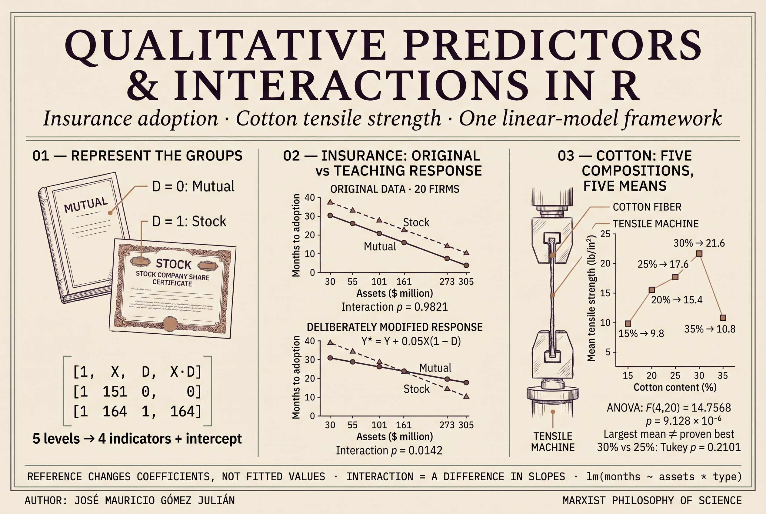
Qualitative Predictors and Interactions in R
01 · What changes when a predictor is qualitative
An insurance company may be mutual or stock-owned; a fiber may be manufactured with different cotton percentages. These differences enter statistical analysis through decisions about what to compare and which relationships to allow. Coding categories represents those decisions: which group supplies the reference, whether slopes must coincide, and whether the relationship between a quantity and the response depends on group membership.
The discussion connects two applications. Insurance data link time to innovation adoption with firm assets and ownership form. Materials data compare tensile strength across five textile compositions. Both cases connect regression, analysis of covariance, and analysis of variance within the general linear model. A model is linear in its parameters; it may contain products of predictors or powers of a variable.
02 · Insurance: question, units, and complete data
Let Y be the elapsed number of months until innovation adoption and X the insurer’s size, measured by assets in millions of dollars. Ownership distinguishes mutual and stock companies. Fewer months indicate faster adoption; because the analyzed response is time, a negative coefficient means a shorter expected waiting time. These teaching data come from the example in Kutner, Nachtsheim, Neter, and Li (2005, pp. 313–318), reproduced in the author’s paper [1–2].
The observational unit is the firm: there are 20 companies, 10 of each type. Recording three attributes does not multiply sample size. Innovation, competition, and profitability provide the economic motivation, while these data support the study of conditional associations. A diffusion mechanism between firms would require temporal or network information, and a causal effect would require additional design and identification assumptions.
| Symbol / code | Definition | Unit / levels |
|---|---|---|
Y / months | Time to adoption | Months |
X / assets | Firm assets | Million dollars |
type | Ownership form | Mutual / Stock |
| D | Indicator for stock company | 0 = mutual; 1 = stock |
| Firm | Months | Assets | Type | D |
|---|---|---|---|---|
| 1 | 17 | 151 | Mutual | 0 |
| 2 | 26 | 92 | Mutual | 0 |
| 3 | 21 | 175 | Mutual | 0 |
| 4 | 30 | 31 | Mutual | 0 |
| 5 | 22 | 104 | Mutual | 0 |
| 6 | 0 | 277 | Mutual | 0 |
| 7 | 12 | 210 | Mutual | 0 |
| 8 | 19 | 120 | Mutual | 0 |
| 9 | 4 | 290 | Mutual | 0 |
| 10 | 16 | 238 | Mutual | 0 |
| 11 | 28 | 164 | Stock | 1 |
| 12 | 15 | 272 | Stock | 1 |
| 13 | 11 | 295 | Stock | 1 |
| 14 | 38 | 68 | Stock | 1 |
| 15 | 31 | 85 | Stock | 1 |
| 16 | 21 | 224 | Stock | 1 |
| 17 | 20 | 166 | Stock | 1 |
| 18 | 13 | 305 | Stock | 1 |
| 19 | 30 | 124 | Stock | 1 |
| 20 | 14 | 246 | Stock | 1 |
The zero-month observation is retained. Its operational meaning—immediate adoption, rounding, or another measurement convention—matters in an actual application. The response is not log-transformed, and no arbitrary constant is added to accommodate zero.
insurance <- data.frame(
  id = 1:20,
  months = c(17,26,21,30,22,0,12,19,4,16,
             28,15,11,38,31,21,20,13,30,14),
  assets = c(151,92,175,31,104,277,210,120,290,238,
             164,272,295,68,85,224,166,305,124,246),
  type = factor(rep(c("Mutual", "Stock"), each = 10),
                levels = c("Mutual", "Stock"))
)
contrasts(insurance$type) <- contr.treatment(levels(insurance$type), base = 1)
stopifnot(nrow(insurance) == 20L, !anyNA(insurance),
          all(table(insurance$type) == 10L))
insurance$D <- as.integer(insurance$type == "Stock")
03 · Indicator functions, factors, and the design matrix
D(Stock) = 1; D(Mutual) = 0
An indicator assigns 1 when a condition holds and 0 otherwise. Zero represents non-membership in the indicated group and remains a valid datum. NA denotes a missing value and NULL a null R object: they are not interchangeable. Factor labels are categories; internal integer codes implement storage. The design matrix contains the columns actually used to fit the model [3–4].
With an intercept and treatment coding, a factor with c observed levels contributes c − 1 columns. Including both an intercept and all c indicators produces an exact dependency because the indicators sum to the column of ones. With two groups, 1 = DMutual + DStock. This concerns independent columns, rather than a general prohibition on including multiple binary variables.
With a full-rank matrix, least-squares coefficients are uniquely identifiable. Under rank deficiency, multiple coefficient vectors may generate the same fitted values: projection onto the column space remains unique. Identification must be assessed in the complete matrix; absent categories or redundant combinations may also cause problems. lm() uses QR decomposition and allows inspection of rank and non-estimable coefficients [5].
contrasts(insurance$type)
X <- model.matrix(~ assets + type, data = insurance)
head(X)
stopifnot(qr(X)$rank == ncol(X))
X_bad <- with(insurance, cbind(Intercept = 1,
  Mutual = as.integer(type == "Mutual"), Stock = D))
c(columns = ncol(X_bad), rank = qr(X_bad)$rank)04 · Assumptions: estimation, inference, and design
The model specifies a conditional mean, E(Y | X, D), with E(ε | X, D) = 0. Classical Gauss–Markov results require full rank and conditional covariance matrix σ²I: constant variance and uncorrelated errors. Conditional normality of errors provides exact finite-sample distributions for classical t and F tests and intervals. Neither the predictors nor the marginal response must be normally distributed.
Companies may share markets, shocks, or ownership links. Such possibilities require substantive information about data collection; a residual plot cannot establish independence. In the textile case, run order, randomization, batches, and machines affect interpretation of the error term. A good numerical fit does not replace a description of the design.
05 · Additive model: differences between parallel lines
For mutual companies, D = 0 and the mean is β0 + β1X. For stock companies, D = 1 and it is (β0 + β2) + β1X. The common slope is a testable restriction; the shift β2 compares ownership groups at the same size. This is also a form of analysis of covariance: comparing groups while adjusting for a continuous covariate.
m_size <- lm(months ~ assets, data = insurance)
m_add <- lm(months ~ assets + type, data = insurance)
summary(m_add)
confint(m_add)
anova(m_size, m_add)
c(n = nobs(m_add), rank = m_add$rank, df = df.residual(m_add),
  SSE = deviance(m_add), MSE = sigma(m_add)^2,
residual_SD = sigma(m_add), R_squared = summary(m_add)$r.squared)| Term | Estimate | Standard error | 95% CI | p |
|---|---|---|---|---|
| Intercept / β₀ | 33.874069 | 1.813858 | [30.047163, 37.700976] | 9.145e-13 |
| Assets / β₁ | -0.101742 | 0.008891 | [-0.120501, -0.082983] | 2.075e-09 |
| Stock − Mutual / β₂ | 8.055469 | 1.459106 | [4.977025, 11.133913] | 3.742e-05 |
ŶStock = 41.929538 − 0.101742X
An additional million dollars in assets is associated with 0.1017 fewer months to adoption, holding ownership type fixed. An increase of 100 million corresponds to 10.1742 fewer months within the linear approximation. At the same size, stock companies have an estimated mean adoption time 8.0555 months longer than mutual companies; the 95% interval for that difference is 4.9770 to 11.1339 months. The intercept refers to X = 0, outside the observed asset range, so it primarily serves as a geometric parameter.
The fit gives SSE = 176.386665, MSE = 10.375686 months², residual standard deviation s = 3.221131 months, and R² = 0.895058. R² summarizes explained variation within this sample; it measures neither causality nor out-of-sample predictive performance. Intervals are two-sided 95% intervals, and p-values use the classical assumptions stated above.
06 · Interaction: allowing slopes to differ
The product XD allows the size–time association to depend on ownership type. The mutual-company slope is β1; the stock-company slope is β1 + β3. Thus β3 estimates the difference in slopes. Retaining X and D alongside XD respects model hierarchy and interprets the interaction in a complete parameterization. The expression assets * type expands the two main terms and their interaction [5].
m_int <- lm(months ~ assets * type, data = insurance)
summary(m_int)
confint(m_int)
anova(m_add, m_int)
linear_contrast <- function(model, L, level = 0.95) {
  stopifnot(length(L) == length(coef(model)), !anyNA(coef(model)))
  estimate <- drop(L %*% coef(model))
  se <- sqrt(drop(L %*% vcov(model) %*% L))
  q <- qt(1 - (1 - level)/2, df.residual(model))
  c(estimate = estimate, SE = se,
    lower = estimate - q * se, upper = estimate + q * se)
}
linear_contrast(m_int, c(0, 0, 1, 150))ŶStock = 41.969620 − 0.101948X
The estimated slope difference is −0.000417 months per million dollars; its 95% CI is [−0.039278, 0.038443]. Testing H₀: β3 = 0 gives F(1,16) = 0.000518 and p = 0.982126. These data provide very little evidence against a common slope. The interval also conveys uncertainty: a large p-value does not establish exact equivalence of slopes.
07 · Changing the reference and centering assets
Changing the reference group changes the coordinates of the representation. In the additive model with stock companies as the reference, the intercept becomes 41.929538 and the mutual-company coefficient becomes −8.055469; the slope remains −0.101742. Fitted values, residuals, SSE, and R² stay the same because the column space is unchanged. relevel() reorders levels; under treatment coding the first is the reference.
With interaction, the group coefficient compares companies at X = 0. It is more useful to center assets at 150 million, a value within both groups’ observed ranges. Defining Xc = X − 150 makes the group coefficient compare firms of that size and the intercept estimate the corresponding mutual-company mean time. Centering does not change the fitted curve.
In the original-response interaction model, Δ(150) = 8.068679 months, with 95% CI [4.651119, 11.486239]. Its variance combines the variances of β̂2 and β̂3 and their covariance. Adding their standard errors is insufficient. In general, for contrast vector L, the standard error is √(Lᵀ V̂ L), where V̂ is the coefficient covariance matrix.
insurance$stock_ref <- relevel(insurance$type, ref = "Stock")
contrasts(insurance$stock_ref) <- contr.treatment(
  levels(insurance$stock_ref), base = 1)
m_ref <- lm(months ~ assets + stock_ref, data = insurance)
insurance$assets_c <- insurance$assets - 150
m_center <- lm(months ~ assets_c * type, data = insurance)
coef(m_ref)
coef(m_center)
stopifnot(isTRUE(all.equal(unname(fitted(m_add)),
                          unname(fitted(m_ref)), tolerance = 1e-10)),
          isTRUE(all.equal(unname(fitted(m_int)),
                          unname(fitted(m_center)), tolerance = 1e-10)))
08 · A teaching modification that makes interaction visible
To see what happens when slopes change, define a response constructed from the original. The modification adds 0.05 months per million dollars of assets only to mutual companies. This is a deliberate teaching operation on the data; it adds no firms and does not represent another empirical study.
β*0 = β0; β*1 = β1 + 0.05; β*2 = β2; β*3 = β3 − 0.05
Because D identifies stock companies, 1 − D identifies mutual companies. The value 0.05 has units of months per million dollars. It is neither a probability, a sampling weight, nor the proportion of mutual firms. In R, == compares values and returns a logical result; as.integer() explicitly converts it to 0 or 1.
# Deliberately modified response: a teaching exercise, not new observations.
insurance$months_demo <- with(insurance,
  months + 0.05 * assets * as.integer(type == "Mutual"))
m_demo_add <- lm(months_demo ~ assets + type, data = insurance)
m_demo_int <- lm(months_demo ~ assets * type, data = insurance)
coef(m_demo_int)
anova(m_demo_add, m_demo_int)
linear_contrast(m_demo_int, c(0, 0, 1, 150))
stopifnot(isTRUE(all.equal(unname(residuals(m_int)),
unname(residuals(m_demo_int)), tolerance = 1e-10)))| Scenario | Mutual slope | Stock slope | Slope difference | Interaction p |
|---|---|---|---|---|
| Original response | −0.101531 | −0.101948 | −0.000417 | 0.982126 |
| Teaching response | −0.051531 | −0.101948 | −0.050417 | 0.014224 |
Comparing the additive and interaction models for Y* gives F(1,16) = 7.564391 and p = 0.014224. The slope difference is detected in the scenario we just constructed. The fitted lines are Ŷ*Mutual = 33.838369 − 0.051531X and Ŷ*Stock = 41.969620 − 0.101948X. Their estimated crossing is around 161.28 million dollars: a property of this exercise, not a causally identified economic threshold.
An instructive algebraic consequence follows. The added term lies in the full model’s column space, so some coefficients change while the full-model residuals remain identical to those from the original response. R² may change because the new response’s total variation also changes. Comparing R² between Y and Y* does not evaluate two models for the same response.
09 · Separate fits, degrees of freedom, and model comparison
Fitting one line per group gives the same group-line coefficients and fitted values as the joint model with full interaction, provided the same records and unweighted least squares are used. Inference may differ: the classical joint fit estimates a common residual variance, while each separate regression estimates its own variance.
group_models <- lapply(levels(insurance$type), function(g)
  lm(months ~ assets, data = insurance, subset = type == g))
names(group_models) <- levels(insurance$type)
sapply(group_models, coef)
sapply(group_models, sigma)
group_fit <- numeric(nrow(insurance))
for (g in names(group_models)) {
  k <- insurance$type == g
  group_fit[k] <- predict(group_models[[g]], newdata = insurance[k, ])
}
stopifnot(max(abs(group_fit - fitted(m_int))) < 1e-8)MSE = SSE / dfres; s = √MSE
| Fit | n | Parameters / rank | Residual df | SSE | s |
|---|---|---|---|---|---|
| Original additive | 20 | 3 | 17 | 176.386665 | 3.221131 |
| Original interaction | 20 | 4 | 16 | 176.380957 | 3.320212 |
| Separate mutual | 10 | 2 | 8 | 111.084407 | 3.726332 |
| Separate stock | 10 | 2 | 8 | 65.296550 | 2.856933 |
Adding an independent column cannot increase SSE for the same sample and response. However, MSE and s may increase because residual degrees of freedom decrease. Here, adding interaction reduces SSE only minimally and increases s. The full model’s pooled variance is an average of group variances weighted by their residual degrees of freedom; it need not be smaller than both.
R denotes the restricted model and F the full model; p is each design matrix’s rank. The numerator measures the average cost of imposing restrictions, and the denominator estimates the full model’s residual variance. With one restriction, F equals the corresponding coefficient’s squared t statistic. Comparison requires nested models, the same response, and the same records. anova(m_add, m_int) tests slopes; anova(m_int) produces a sequential decomposition that may depend on term order [6].
10 · Diagnostics: residuals, leverage, and influence
A residual ei = yi − ŷi measures vertical discrepancy from the fit. Leverage hii depends on predictors and the design matrix. Influence evaluates how much the fit changes when an observation is removed. A firm with extreme assets may have high leverage and a small residual; another may have a large residual with moderate leverage. Neither characteristic alone determines overall influence.
ri = ei / [s√(1 − hii)]
Cooki = [ei² / (p s²)] · [hii / (1 − hii)²]
These expressions assume full-rank least squares, p parameters, and estimable residual variance. Under homoscedasticity, Var(e | X) = σ²(I − H): raw residuals do not all have equal variance and are not independent, even when the errors satisfy the model. Standardization accounts for this geometric effect. rstudent() uses a dispersion estimate that excludes the observation being evaluated [7–8].
| Plot | Question it addresses |
|---|---|
| Residuals / fitted | Is systematic mean structure left over? |
| Normal Q–Q | Is residual shape compatible with normality? |
| Scale–Location | Does spread change with the fitted level? |
| Residuals / leverage | Do discrepancy and leverage combine? |
| Firm | Residual | Standardized residual | hᵢᵢ | Cook |
|---|---|---|---|---|
| 6 | -5.6915 | -1.9623 | 0.1892 | 0.2995 |
| 10 | 6.3406 | 2.1183 | 0.1365 | 0.2364 |
| 17 | -5.0403 | -1.6553 | 0.1064 | 0.1087 |
| 14 | 2.9889 | 1.0525 | 0.2227 | 0.1058 |
| 3 | 4.9308 | 1.6138 | 0.1003 | 0.0968 |
Firms 6 and 10 have Cook distances of about 0.2995 and 0.2364. The heuristic 4/n = 0.20 flags them for investigation; the threshold 2p/n = 0.30 flags no extreme leverage in this fit. These are exploratory rules, not tests or instructions to delete data. The largest Cook distance is below 0.5, which does not remove the need to examine measurement, provenance, and sensitivity of conclusions.
diagnostics <- data.frame(id = insurance$id,
  residual = residuals(m_add), standardized = rstandard(m_add),
  studentized = rstudent(m_add), leverage = hatvalues(m_add),
  Cook = cooks.distance(m_add))
diagnostics[order(diagnostics$Cook, decreasing = TRUE), ]
influence.measures(m_add)
hc3_vcov <- function(model) {
  Z <- model.matrix(model)
  stopifnot(qr(Z)$rank == ncol(Z))
  bread <- solve(crossprod(Z))
  u <- residuals(model)/(1 - hatvalues(model))
  bread %*% crossprod(Z, Z * as.vector(u^2)) %*% bread
}
cbind(estimate = coef(m_add), classical_SE = sqrt(diag(vcov(m_add))),
      HC3_SE = sqrt(diag(hc3_vcov(m_add))))
# Sensitivity analysis: retain the original fit as the main analysis.
sensitivity <- lapply(c(6L, 10L), function(k)
  coef(lm(months ~ assets + type, data = insurance,
          subset = id != k)))
names(sensitivity) <- c("omit_6", "omit_10")
sensitivity
The laboratory adds HC3 standard errors as a heteroscedasticity sensitivity analysis. It computes (XᵀX)⁻¹ Xᵀ diag[eᵢ²/(1 − hᵢᵢ)²] X (XᵀX)⁻¹. OLS coefficients remain unchanged; their estimated covariance changes. HC3 does not repair a misspecified mean, causal confounding, or dependence between firms. With 20 observations, robust inference still requires care about small-sample approximation.
| Term | Classical SE | HC3 SE |
|---|---|---|
| Intercept | 1.813858 | 1.311688 |
| Assets | 0.008891 | 0.009051 |
| Stock − Mutual | 1.459106 | 1.699138 |
11 · A minimal sensitivity experiment
Consider six points on y = x, with x = (1, 2, 3, 4, 5, 20). Increase y by four units first at x = 3 and then at x = 20, leaving the other observations unchanged. Perturbation size is identical; the point’s position in the design differs. The x = 20 point has leverage 0.9668, whereas x = 3 has leverage 0.1987.
toy <- data.frame(x = c(1,2,3,4,5,20), y = c(1,2,3,4,5,20))
toy$y_near <- toy$y
toy$y_far <- toy$y
toy$y_near[3] <- toy$y_near[3] + 4
toy$y_far[6] <- toy$y_far[6] + 4
toy_base <- lm(y ~ x, data = toy)
toy_near <- lm(y_near ~ x, data = toy)
toy_far <- lm(y_far ~ x, data = toy)
data.frame(x = toy$x, leverage = hatvalues(toy_base))
rbind(original = coef(toy_base), near = coef(toy_near), far = coef(toy_far))
# The exact baseline has SSE=0: do not interpret Cook's D for that fit.The example demonstrates a geometric property of least squares. The distant point is not automatically invalid: it may be a valuable observation extending the study range. Applied assessment combines geometry, discrepancy, record quality, and knowledge of the process.
12 · Prediction and uncertainty for a firm
A conditional mean and a future observation have different uncertainties. For a design row x₀, a mean confidence interval uses s√[x₀ᵀ(XᵀX)⁻¹x₀]. An individual prediction interval uses s√[1 + x₀ᵀ(XᵀX)⁻¹x₀]: it adds variation of a new response around its mean. Both use the appropriate t quantile under the classical assumptions [9].
new_firms <- data.frame(assets = rep(150, 2),
  type = factor(c("Mutual", "Stock"), levels = levels(insurance$type)))
predict(m_add, newdata = new_firms, interval = "confidence")
predict(m_add, newdata = new_firms, interval = "prediction")| Type | Estimated mean | 95% mean CI | 95% individual PI |
|---|---|---|---|
| Mutual | 18.6128 | [16.4349, 20.7906] | [11.4763, 25.7492] |
| Stock | 26.6682 | [24.3600, 28.9765] | [19.4909, 33.8455] |
Observed assets range from 31 to 290 million for mutual companies and from 68 to 305 million for stock companies. Between-group comparisons have common support from 68 to 290 million. Far extrapolations may yield negative times, revealing a limitation of this approximation to a nonnegative duration. Censoring, unobserved adoption events, or strong asymmetry motivate duration models; a Gamma distribution with log link requires strictly positive responses and does not directly accommodate the zero observed here.
13 · Materials: fiber composition and tensile strength
The second case studies fibers in a blend containing cotton. The predictor is cotton percentage by weight: 15, 20, 25, 30, and 35%, with five strength measurements per level. The physical variable is quantitative; it can be represented as a factor when the aim is to estimate an unrestricted mean for each tested level. The data and their interpretation are verified against Penn State’s teaching example on textile strength [10].
| Cotton (%) | Strength observations (lb/in²) | n | Mean |
|---|---|---|---|
| 15 | 7, 7, 15, 11, 9 | 5 | 9.8 |
| 20 | 12, 17, 12, 18, 18 | 5 | 15.4 |
| 25 | 14, 18, 18, 19, 19 | 5 | 17.6 |
| 30 | 19, 25, 22, 19, 23 | 5 | 21.6 |
| 35 | 7, 10, 11, 15, 11 | 5 | 10.8 |
The experimental unit is the fiber or material unit assigned a composition; a causal interpretation of treatment differences requires randomized execution, independent replicates, and control of other conditions. Five readings on one specimen would not equal five independent replicates. The identifier treatment denotes composition levels, rather than presupposing five different mechanical test types.
cotton <- data.frame(
  percent = rep(c(15,20,25,30,35), each = 5),
  strength = c(7,7,15,11,9, 12,17,12,18,18,
               14,18,18,19,19, 19,25,22,19,23, 7,10,11,15,11)
)
cotton$treatment <- factor(cotton$percent, levels = c(15,20,25,30,35))
contrasts(cotton$treatment) <- contr.treatment(
  levels(cotton$treatment), base = 1)
stopifnot(nrow(cotton) == 25L, !anyNA(cotton))
aggregate(strength ~ treatment, data = cotton, FUN = mean)
# Safe conversion of numeric-looking labels, not the internal factor codes:
stopifnot(identical(as.numeric(as.character(cotton$treatment)),
                    cotton$percent))
To recover numerical values from labels such as “15” and “20”, use as.numeric(as.character(factor)). Applying as.numeric() directly to the factor returns internal codes 1, 2, 3, 4, and 5. A factor represents one categorical variable with multiple levels; it needs no second variable in order to be created. Explicit coercion can convert numeric text to numbers, while unparseable strings produce missing values with a warning [4].
14 · Five means, four indicators, and one fit
Y = α + δ20D20 + δ25D25 + δ30D30 + δ35D35 + ε
The first form assigns a separate mean to each level. In the second, 15% is the reference: α = μ15 and δj = μj − μ15. Estimated coefficients are α̂ = 9.8, δ̂20 = 5.6, δ̂25 = 7.8, δ̂30 = 11.8, and δ̂35 = 1.0. Reconstruct a mean by adding the intercept and its corresponding difference; for example, μ̂30 = 9.8 + 11.8 = 21.6.
| Level | Intercept | D₂₀ | D₂₅ | D₃₀ | D₃₅ |
|---|---|---|---|---|---|
| 15 | 1 | 0 | 0 | 0 | 0 |
| 20 | 1 | 1 | 0 | 0 | 0 |
| 25 | 1 | 0 | 1 | 0 | 0 |
| 30 | 1 | 0 | 0 | 1 | 0 |
| 35 | 1 | 0 | 0 | 0 | 1 |
The factor, four manual indicators, and five indicators without an intercept generate the same fitting space. They therefore yield the same fitted values, residuals, SSE, and R²; the last parameterization estimates the five means directly. The word class can denote a group here without imposing countability or a universal hierarchy. An indicator vector represents group membership; it does not create a new ontological class of observations.
m_factor <- lm(strength ~ treatment, data = cotton)
m_cell <- lm(strength ~ 0 + treatment, data = cotton)
cotton$D20 <- as.integer(cotton$treatment == "20")
cotton$D25 <- as.integer(cotton$treatment == "25")
cotton$D30 <- as.integer(cotton$treatment == "30")
cotton$D35 <- as.integer(cotton$treatment == "35")
m_manual <- lm(strength ~ D20 + D25 + D30 + D35, data = cotton)
m_linear <- lm(strength ~ percent, data = cotton)
m_quadratic <- lm(strength ~ percent + I(percent^2), data = cotton)
summary(m_factor)
anova(m_factor)
confint(m_factor)
coef(m_cell)
anova(m_linear, m_factor)       # linear lack of fit: 3 restrictions
anova(m_quadratic, m_factor)    # quadratic lack of fit: 2 restrictions
stopifnot(max(abs(fitted(m_factor) - fitted(m_manual))) < 1e-10,
          max(abs(fitted(m_factor) - fitted(m_cell))) < 1e-10)
15 · ANOVA: partitioning variation to compare means
SSB = Σj nj(ȳj − ȳ)²; SSE = ΣjΣi(yij − ȳj)²
SST = SSB + SSE; F = [SSB / (c − 1)] / [SSE / (n − c)]
SST measures variation around the overall mean; SSB captures differences between composition means; SSE captures variation within each composition. Under H₀: μ15 = μ20 = μ25 = μ30 = μ35, both mean squares estimate the same variance. Their ratio is compared with F(4,20) under the classical assumptions. Although the method analyzes variances, its central question concerns equality of population means.
| Source | Sum of squares | df | Mean square | F | p |
|---|---|---|---|---|---|
| Composition | 475.76 | 4 | 118.94 | 14.756824 | 9.128e−6 |
| Error | 161.20 | 20 | 8.06 | — | — |
| Total | 636.96 | 24 | — | — | — |
The test rejects global equality of means at the 0.05 level. Residual standard deviation is √8.06 = 2.839014 lb/in² and R² = 0.746923. In this one-factor design, η² = SSB/SST = 0.746923 equals R² as a description of the sample. It is neither a percentage of a demonstrated causal mechanism nor a removal of estimation uncertainty.
The largest observed mean occurs at 30% cotton. Claiming that it exceeds another level requires a comparison with uncertainty and attention to the number of comparisons performed. A significant global test does not establish a difference for every pair.
16 · Percentage as a number or factor: different restrictions
A straight line treats percentage increases as changes governed by a common slope. A quadratic admits curvature while remaining linear in its coefficients. The factor model permits five means without specifying a continuous shape between levels. The choice depends on the scientific question and whether the restrictions describe the data.
E(Y | x) = a + bx + cx²
E(Y | level = j) = μj
| Model | Rank | SSE | R² | Lack-of-fit F vs. factor | p |
|---|---|---|---|---|---|
| Linear | 2 | 603.340000 | 0.052782 | 18.285360 (3,20) | 5.967e−6 |
| Quadratic | 3 | 260.125714 | 0.591614 | 6.136831 (2,20) | 0.008353 |
| Factor | 5 | 161.200000 | 0.746923 | — | — |
Five replicates per level allow pure error estimation through the factor model. A lack-of-fit test compares that error with the extra variation left by a restricted shape. Both the line and the parabola show detectable lack of fit at the 0.05 level. An unconvincing linear slope does not imply absence of a relationship: it may indicate that the proposed shape misses a substantial decline in strength.
17 · Multiple comparisons and interval interpretation
Five means generate ten pairwise comparisons. If the question concerns that entire family, Tukey adjusts inference to control the family-wise error rate under classical ANOVA. Simultaneous intervals have 95% joint coverage, unlike ten pointwise intervals treated as a single claim [11].
cotton_aov <- aov(strength ~ treatment, data = cotton)
TukeyHSD(cotton_aov, "treatment", conf.level = 0.95)
mean_grid <- data.frame(treatment = factor(c(15,20,25,30,35),
                         levels = levels(cotton$treatment)))
predict(m_factor, newdata = mean_grid, interval = "confidence")| Pair (% cotton) | Difference (lb/in²) | Simultaneous 95% CI | Adjusted p |
|---|---|---|---|
| 20 − 15 | 5.60 | [0.2270, 10.9730] | 0.0385 |
| 25 − 15 | 7.80 | [2.4270, 13.1730] | 0.002595 |
| 30 − 15 | 11.80 | [6.4270, 17.1730] | 1.901e-05 |
| 35 − 15 | 1.00 | [-4.3730, 6.3730] | 0.9798 |
| 25 − 20 | 2.20 | [-3.1730, 7.5730] | 0.7372 |
| 30 − 20 | 6.20 | [0.8270, 11.5730] | 0.01889 |
| 35 − 20 | -4.60 | [-9.9730, 0.7730] | 0.1163 |
| 30 − 25 | 4.00 | [-1.3730, 9.3730] | 0.2101 |
| 35 − 25 | -6.80 | [-12.1730, -1.4270] | 0.009065 |
| 35 − 30 | -10.80 | [-16.1730, -5.4270] | 6.241e-05 |
The 30% − 25% contrast estimates 4.0 lb/in², with interval [−1.3730, 9.3730] and adjusted p = 0.2101. Thus the largest mean at 30% does not establish superiority over 25% under this adjustment. By contrast, 30% − 35% estimates 10.8 lb/in², with interval [5.4270, 16.1730] and adjusted p ≈ 0.0000624. Failing to reject a difference does not establish equivalence: equivalence requires margins and a procedure designed for that question.
With heterogeneous variances, the validity of pooled ANOVA and Tukey comparisons should be reconsidered. Depending on design, Welch ANOVA with compatible comparisons, a variance model, or robust inference may be appropriate. Batches or repeated measurements require a dependence structure. No automatic correction replaces that substantive decision.
18 · What the two cases support
In insurance, assets are negatively associated with adoption time, and ownership form is associated with a size-adjusted level difference. The original data provide little evidence of different slopes. The teaching modification examines an explicitly introduced interaction and shows why interpretation must depend on the response actually analyzed.
In materials, composition is associated with strength differences that a straight line does not adequately describe. The factor preserves five means and exposes the connection between regression and ANOVA. Multiple comparison distinguishes the largest observed average from a statistically supported difference for a specific pair.
Both cases show that coding selects a testable representation. Changing the reference preserves predictions; imposing a common slope changes restrictions; transforming the response changes the analytical object. Scientific interpretation requires distinguishing those operations, examining uncertainty, and reconstructing the material conditions under which data were produced.
19 · Reproducing the analysis and figures
R blocks appear in execution order and use only base R and its standard packages. All data are included. Copy them sequentially into one script without additional input files. Group codes stay in English (Mutual, Stock) so both language versions execute exactly the same analysis. Reported numbers were recomputed using least squares and t, F, and studentized-range distributions; minor rounding differences do not change the conclusions.
The following block saves data, diagnostics, PDF plots, and session information in a folder relative to the working directory. This article’s figures are drawn from the same data and models. Documenting a new study would additionally require provenance, a measurement protocol, software versions, and exclusion criteria before interpreting results.
outdir <- "predictores_resultados"
dir.create(outdir, showWarnings = FALSE)
write.csv(insurance, file.path(outdir, "insurance.csv"), row.names = FALSE)
write.csv(cotton, file.path(outdir, "cotton.csv"), row.names = FALSE)
write.csv(diagnostics, file.path(outdir, "diagnostics.csv"), row.names = FALSE)
pdf(file.path(outdir, "diagnostics.pdf"), width = 8, height = 8)
par(mfrow = c(2,2))
plot(m_add, which = c(1,2,3,5), ask = FALSE)
plot(m_factor, which = c(1,2,3,5), ask = FALSE)
dev.off()
pdf(file.path(outdir, "cases.pdf"), width = 8, height = 6)
plot(months ~ assets, data = insurance, pch = 16 + insurance$D,
     col = c("#8b4513", "#554637")[1 + insurance$D])
b <- coef(m_add)
abline(b[1], b[2], col = "#8b4513")
abline(b[1] + b[3], b[2], col = "#554637", lty = 2)
legend("topright", levels(insurance$type), pch = c(16,17),
       col = c("#8b4513", "#554637"), lty = c(1,2), bty = "n")
plot(months_demo ~ assets, data = insurance, pch = 16 + insurance$D)
b <- coef(m_demo_int)
abline(b[1], b[2], col = "#8b4513")
abline(b[1] + b[3], b[2] + b[4], col = "#554637", lty = 2)
boxplot(strength ~ treatment, data = cotton, col = "#fffdf7",
        xlab = "Cotton percentage", ylab = "Tensile strength")
plot(TukeyHSD(cotton_aov, "treatment"), las = 1)
dev.off()
capture.output(sessionInfo(), file = file.path(outdir, "sessionInfo.txt"))
20 · References and documentation
- José Mauricio Gómez Julián (2021). Variables cualitativas e interacciones. 24-page paper, published under the pseudonym Isadore Nabi. Read.
- Kutner, M. H., Nachtsheim, C. J., Neter, J., & Li, W. (2005). Applied Linear Statistical Models, 5th ed. McGraw-Hill/Irwin. Chapter 8, pp. 313–318.
- R Core Team.
model.matrix: constructing design matrices. Read. - R Core Team.
factor: levels, labels, and coercion. Read. - R Core Team.
lm: linear models and formulas. Read. - R Core Team.
anova.lm: sequential tables and nested comparisons. Read. - R Core Team.
plot.lm: diagnostic plots. Read. - R Core Team.
influence.measures: residuals, leverage, and case deletion. Read. - R Core Team.
predict.lm: confidence and prediction intervals. Read. - Penn State, Department of Statistics. STAT 503, Lesson 03: Experiments with a Single Factor. Fiber-strength example with different cotton percentages. Read.
- R Core Team.
TukeyHSD: simultaneous mean comparisons. Read.
R references point to official documentation consulted on November 4, 2026. The insurance example preserves the observations in the source paper; the complete textile table is cross-checked against the university source listed above. The modified response is consistently identified as a teaching construction.
Leave a Comment/Deja un Comentario