
Mathematics · R Programming · Discrete Dynamical Systems
The Collatz Conjecture as a Custom Function in R
An introduction to functions, iteration, and recursion through an extraordinarily simple mathematical rule whose global behavior continues to resist a general proof.
A particularly pleasant example of a custom function is one built to study the celebrated Collatz conjecture computationally. The choice is useful because the mathematical rule is very simple, whereas its global behavior is not: one need only distinguish between even and odd numbers and repeatedly apply the same transformation. This combination allows us to concentrate on programming logic without losing sight of the mathematical object being programmed.
In elementary terms, the conjecture states that if we begin with any positive integer and divide it by two when it is even, or multiply it by three and add one when it is odd, the resulting sequence will eventually reach one. It is important to formulate this carefully: a program can verify that this happens for a particular starting value—or for a finite collection of values—but such computational verification does not, by itself, constitute a proof that it happens for every positive integer. That is precisely where the mathematical problem lies.
1. The Collatz rule and what it means to verify it
Mathematically, the rule generating successive images can be expressed by the following piecewise-defined function:
| Condition | Operation | New image |
|---|---|---|
| n is even | Divide by 2 | T(n) = n/2 |
| n is odd | Multiply by 3 and add 1 | T(n) = 3n + 1 |
Table 1. The local Collatz rule. Each step is completely determined by the parity of the present state.
If we begin from an origin or seed value n0, successive applications of the function construct an orbit:
This notation lets us introduce from the outset a distinction that will later matter in R. If the orbit reaches one for the first time after k applications of the rule, then k iterations or transitions have occurred, whereas the complete list of states contains k + 1 values, because the starting value is counted as well.
The total stopping time may be defined as the number of applications of T required to reach 1. If it is denoted by τ(n), the conjecture can be written compactly as: τ(n) < ∞ for every positive integer n.
Consequently, what we shall program below is not a “proof” of the conjecture in the mathematical sense of a universal demonstration. It will instead be a mechanism capable of generating and examining particular orbits, recording their states, and counting how many transformations were required to reach 1 whenever that value is indeed reached.
2. A first custom function in R
To construct the preceding rule in R, it is useful to recall that a custom function can take an input, subject it to a set of instructions, and return an output. At this first stage there will be no iteration yet: a single number will be evaluated and its next Collatz image produced.
The fundamental condition is parity. In R, the operator %% returns the remainder of a division. If n %% 2 == 0, the number is divisible by two and is therefore even. If the remainder is nonzero, it is odd.
R · one-step ruleCollatzFunction <- function(n) {
  if (length(n) != 1L || !is.finite(n) || n < 1 || n != floor(n)) {
    stop("n must be a positive integer.")
  }

  if (n %% 2 == 0) {
    j <- n / 2
  } else {
    j <- 3 * n + 1
  }

  return(j)
}
The function receives a positive integer n, determines whether it is even or odd, and stores the result in j. The instruction return(j) does not, strictly speaking, mean “print j on the screen”; it means that j will be the value returned by the function. When the function is run directly in R’s interactive console, that returned value is usually displayed automatically, which explains why the two ideas can easily be confused when one is beginning to program.
return(x) terminates the function and supplies x as its result. print(x), by contrast, explicitly requests that x be printed. A function can return a value without containing any print() instruction.
Notice also that there is no need to prevent this function from being evaluated at 1: under the standard rule, 1 is odd and its next image would be 4. What the algorithm constructed below will do is stop the orbit upon reaching 1; that is, it will not apply the rule again once the target has been reached.
3. From a single step to an iterative algorithm
The preceding function performs only one transformation. To obtain a complete orbit, it must be repeated while the current value differs from 1. Here we encounter the “while” loop—while-loop—whose logic is exactly what its name suggests: execute a given block of instructions for as long as a condition remains true.
This second function is therefore iterative. It is not recursive yet, because it does not call itself; rather, it explicitly repeats a block of code by means of while().
R · iterative algorithmIterativeCollatzAlgorithm <- function(m, max_iter = 1000000L) {
  if (length(m) != 1L || !is.finite(m) || m < 1 || m != floor(m)) {
    stop("m must be a positive integer.")
  }

  trajectory <- m
  iterations <- 0L

  while (m != 1) {
    if (iterations >= max_iter) {
      stop("max_iter was reached before 1.")
    }

    m <- CollatzFunction(m)
    trajectory <- c(trajectory, m)
    iterations <- iterations + 1L
  }

  return(trajectory)
}
The logic is simple. The vector trajectory is created inside the function itself and initially contains the seed value. Then, each time the loop runs, m is replaced by its next image and that new value is appended to the end of the vector. When m reaches 1, the condition m != 1 ceases to hold and the loop terminates.
The letter m is used here simply to distinguish visually the argument of this second function from the n used in the first. There is no syntactic need to do so: arguments and objects created inside each function have their own local scope, so two different functions may use an argument called n without conflict.
Defining the vector inside the function has an important advantage: each execution retains its own state and does not depend on objects already present in R’s global environment. In other words, if the function is run once with 27 and then with 8, the second orbit does not inherit values from the first.
The argument max_iter is not part of the Mathematics of Collatz; it is a computational precaution. Since the general statement one wishes to prove cannot simply be assumed when writing the program, it is prudent to prevent a loop from continuing without limit if it is used with unexpected data or a modified implementation.
| Object | Type | Role |
|---|---|---|
| CollatzFunction | function | Computes a single image under the Collatz rule. |
| IterativeCollatzAlgorithm | function | Repeats the rule with while() and constructs the complete trajectory down to 1. |
| trajectory | numeric vector | Exists locally during one execution and stores the states visited. |
Table 2. A conceptual equivalent of what would be observed in the R environment after defining the functions. The trajectory vector need not remain in the global environment.
4. The orbit of 27: 112 states and 111 iterations
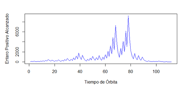
We can now evaluate any number in the algorithm we have constructed. Take the classic example of 27. The sequence begins 27, 82, 41, 124, 62, 31… and continues through rises and falls until it finally reaches 1.
R · exampleorbit_27 <- IterativeCollatzAlgorithm(27)
length(orbit_27)
# 112

length(orbit_27) - 1L
# 111

max(orbit_27)
# 9232
This is a good place to make the terminology precise. The stored orbit contains 112 states, because it includes both the starting point 27 and the endpoint 1. However, between 112 states there are only 111 transitions. Consequently, the total stopping time of 27, understood as the number of applications of the rule required to reach one, is 111.
| k=027 | k=182 | k=241 | k=3124 | k=462 | k=531 | k=694 | k=747 |
| k=8142 | k=971 | k=10214 | k=11107 | k=12322 | k=13161 | k=14484 | k=15242 |
| k=16121 | k=17364 | k=18182 | k=1991 | k=20274 | k=21137 | k=22412 | k=23206 |
| k=24103 | k=25310 | k=26155 | k=27466 | k=28233 | k=29700 | k=30350 | k=31175 |
| k=32526 | k=33263 | k=34790 | k=35395 | k=361186 | k=37593 | k=381780 | k=39890 |
| k=40445 | k=411336 | k=42668 | k=43334 | k=44167 | k=45502 | k=46251 | k=47754 |
| k=48377 | k=491132 | k=50566 | k=51283 | k=52850 | k=53425 | k=541276 | k=55638 |
| k=56319 | k=57958 | k=58479 | k=591438 | k=60719 | k=612158 | k=621079 | k=633238 |
| k=641619 | k=654858 | k=662429 | k=677288 | k=683644 | k=691822 | k=70911 | k=712734 |
| k=721367 | k=734102 | k=742051 | k=756154 | k=763077 | k=779232 | k=784616 | k=792308 |
| k=801154 | k=81577 | k=821732 | k=83866 | k=84433 | k=851300 | k=86650 | k=87325 |
| k=88976 | k=89488 | k=90244 | k=91122 | k=9261 | k=93184 | k=9492 | k=9546 |
| k=9623 | k=9770 | k=9835 | k=99106 | k=10053 | k=101160 | k=10280 | k=10340 |
| k=10420 | k=10510 | k=1065 | k=10716 | k=1088 | k=1094 | k=1102 | k=1111 |
Table 3. Complete orbit of 27. The label k indicates how many applications of the rule have been performed. The maximum, 9232, appears at k = 77; one appears at k = 111.
The trajectory also reveals a property that makes the problem so suggestive: an extraordinarily simple deterministic rule does not necessarily generate a visually simple evolution. The fact that the system is perfectly determined step by step does not mean that its global behavior is obvious.
If one wishes to retain the traditional graph in R, it can be generated, for example, with:
R · optional visualizationplot(
  orbit_27,
  type = "l",
  xlab = "Iteration k",
  ylab = "n_k"
)
The table presents the complete orbit so that each state can be read directly and followed step by step.
5. A second solution: recursion
There is another way to design the algorithm. It may be somewhat less intuitive when first imagined, but it has a notable elegance: instead of constructing a while() loop, the function itself calls itself again after calculating the next value.
The problem now requires a function with two principal characteristics: its input is a positive integer representable by the numerical system being used; its output contains, on the one hand, the trajectory followed and, on the other, the number of transformations performed in order to reach one.
R · recursive versionRecursiveCollatz <- function(n, v = NULL) {
  if (length(n) != 1L || !is.finite(n) || n < 1 || n != floor(n)) {
    stop("n must be a positive integer.")
  }

  v <- c(v, n)

  if (n == 1) {
    return(list(
      steps = v,
      iterations = length(v) - 1L
    ))
  }

  if (n %% 2 == 0) {
    n <- n / 2
  } else {
    n <- 3 * n + 1
  }

  return(RecursiveCollatz(n, v))
}
Here recursion is used in the precise programming sense: during the execution of RecursiveCollatz(), a new call to RecursiveCollatz() appears. That new call receives a different value of n and an enlarged copy of the vector v.
The condition n == 1 is the base case. Without a reachable base case, a recursive definition would continue producing additional calls until the available resources were exhausted. When 1 is reached, no new call is created: the list containing the orbit and the number of iterations is returned.
c() concatenates elements or vectors. list() constructs a list whose components may have different names and types. length() returns the number of elements in an object such as a vector or list; it should not be confused with dim(), which reports the dimensions of objects that possess a dimensional attribute.
The expression iterations = length(v) – 1L deserves attention. If v contains both the initial value and the final one, its length counts states, not transformations. Subtracting one corrects exactly that difference.
| Seed | Returned states | Iterations |
|---|---|---|
| 8 | 8 → 4 → 2 → 1 | 3 |
| 27 | 112 states from 27 to 1 | 111 |
Table 4. The difference between counting states and counting applications of the function. In the trajectory 8 → 4 → 2 → 1 there are four values, but only three steps.
A practical qualification must be added. Recursion is an excellent tool for understanding the logical structure of the problem, but it is not always the most robust way to traverse long orbits in R: each recursive call adds a new execution frame, and the available depth is finite. For intensive computational work, the iterative version is usually preferable; for understanding what it means for a function to invoke itself, the recursive version is particularly transparent.
6. How to think about recursion mathematically
Before programming a recursive solution, it is useful to separate two things which, although intimately related, are not identical: the mathematical dynamics and the program’s call structure. The fundamental mathematical function remains T. What changes is the way in which the program organizes the calculation of its iterations.
The algorithm can be thought of as follows:
| Logical step | Action |
|---|---|
| 1 | Enter a positive integer N. |
| 2 | Record N as a new state of the trajectory. |
| 3 | If N = 1, return the trajectory and terminate. |
| 4a | If N is even, assign N ← N/2. |
| 4b | If N is odd, assign N ← 3N + 1. |
| 5 | Execute the same function again using the new value of N. |
Table 5. Use case for the recursive solution. Recursion appears in the last step: the function is executed again with a new input.
Mathematically, however, there is no need to define a new function C(n) whose value is always 1 whenever the recursion terminates. Such a notation would conceal the object that actually matters. It is cleaner to retain T as the Collatz map and define the orbit through successive iterations:
The total stopping time may then be written as the first index at which the orbit reaches one:
This formulation makes the real difficulty visible. We know exactly the local rule that takes one state to the next. What does not follow automatically from that definition is that τ(n) is finite for every positive integer.
Take n = 8:
| k = 0 | k = 1 | k = 2 | k = 3 | |||
|---|---|---|---|---|---|---|
| 8 | → | 4 | → | 2 | → | 1 |
Table 6. From 8 to 1 there are four states and three applications of T. Therefore, τ(8) = 3.
The recursive function reproduces this same chain computationally, but each arrow now corresponds not only to a mathematical transformation but also to a new function call. The mathematical sequence advances from 8 to 4, from 4 to 2, and from 2 to 1; meanwhile, the program creates successive execution levels until it encounters the base case.
7. The call stack: why it is LIFO
To understand what happens during recursion, we can use a deliberately simple example. Suppose there is a “Listing X” with the following instructions:
1. Execute A1.
2. Execute A2.
3. Execute the instructions in Listing X.
4. Return and print “Hello, Fernanda”.
Upon reaching step 3, the program begins another execution of the same listing. That new execution reaches its own step 3 and creates another, and so on. Because there is no base case here, step 4 is never executed: the resources that the environment permits for nested calls will be exhausted first.
| Level | A1 | A2 | Step 3 | Result |
|---|---|---|---|---|
| Listing X₀ | executes | executes | calls X₁ | remains pending |
| Listing X₁ | executes | executes | calls X₂ | remains pending |
| Listing X₂ | executes | executes | calls X₃ | remains pending |
| ⋮ | ⋮ | ⋮ | ⋮ | ⋮ |
Table 7. Structure of recursive calls. Each call is suspended while it waits for the call created within it to finish.
When a base case does exist, as in our algorithm when 1 is reached, the situation changes. The deepest call terminates first; then the call that created it can terminate; then the preceding one, and so on. This is why the natural structure of nested calls is a stack, organized as LIFO: Last In, First Out.
| TOP OF STACK · call with n = 1 · terminates first |
| call with n = 2 · waits for the result of n = 1 |
| call with n = 4 · waits for the result of n = 2 |
| BASE · call with n = 8 · created first |
Table 8. The call stack for 8 → 4 → 2 → 1. The call with 1 is the last to enter and the first able to finish; the pending calls are then resolved in reverse order.
The analogy with a stack of plates remains useful: if several plates are stacked one on top of another, the last one placed sits at the top and is the first that can be removed without dismantling the stack. It is nevertheless useful to specify the technical reason: recursive calls are organized in this way because of the nested structure of program control. The relationship with memory locality or possible cache effects may matter in other performance contexts, but it is not what explains why the call stack is LIFO.
8. What Collatz teaches us about Mathematics and Computation
There is still a conceptual question that deserves attention. At first glance, it might seem that the mathematical formulation offers us a “continuous” process whereas the program turns it into a collection of discrete steps. That opposition, however, does not correctly describe this problem. Collatz dynamics are discrete in the mathematical definition itself: iteration time is indexed by 0, 1, 2, 3, … and each state belongs, in the usual formulation, to the set of positive integers.
The interesting difference, therefore, is not between continuous Mathematics and discrete Computation. It lies elsewhere: between defining a rule, calculating its consequences for particular cases, and proving a global property of all its orbits.
| Level | What we know | What does not follow automatically |
|---|---|---|
| Mathematical rule | For each state, we know exactly what the next one is. | From this alone, we do not know the global fate of every possible orbit. |
| Computational calculation | We can follow a particular orbit step by step and verify whether it reaches 1. | A finite number of verifications is not equivalent to a universal proof. |
| Mathematical proof | It would seek to establish a proposition valid for every positive integer. | It cannot simply be replaced by enumerating more and more cases. |
Table 9. Three levels of knowledge that Collatz forces us to distinguish: local specification, computational experimentation, and global proof.
This distinction allows us to formulate more precisely the epistemological reflection that makes the example attractive. Mathematics does not necessarily consist in placing a phenomenon inside an analytical form whose behavior is already known. Collatz shows exactly the opposite: we can possess a perfectly defined rule and still lack a complete characterization of its global behavior.
Nor can Computation be reduced to attending to “particularities” that Mathematics has supposedly abstracted away. Here both operate on the same discrete object, but they ask different questions. The program allows us to execute the rule, inspect orbits, measure stopping times, discover regularities, and subject auxiliary conjectures to numerical testing. Mathematical proof, by contrast, asks what can necessarily be asserted for an infinite class of cases.
This is probably one of the most interesting lessons that can be drawn from the problem from the joint perspective of Mathematics and Computer Science. In Collatz there is local determination, effective computability of every step, and an enormous body of evidence for particular values; but those three things must not be confused with a universal proof.
9. A precaution: mathematical integers are not machine integers
Finally, there is an additional difference between the mathematical object and its concrete implementation that should be made explicit. The expression “any N ∈ ℕ” describes an unlimited mathematical domain. A computer, by contrast, represents numbers by means of finite structures.
Base R includes, among other things, values of type integer, whose range is limited, and numeric values, which normally use double-precision arithmetic. The latter can represent all integers exactly only up to a certain size; above 253, not every consecutive integer has an exact representation as a double-precision number.
The issue is particularly relevant in Collatz because an orbit can grow far above its initial value before beginning to descend. Consequently, an implementation intended to investigate very large numbers must use exact integer arithmetic of greater capacity—for example, arbitrary-precision integers—and carefully check for possible overflow or loss of exactness.
Mathematical object: T acts on all positive integers.
Concrete program: it can operate correctly only on values that its numerical representation and memory resources can manipulate exactly.
This does not invalidate the pedagogical use of the preceding code. For small seeds such as 8 or 27, the implementation is perfectly adequate. What it prevents is our attributing to a finite computational representation the same unlimited domain possessed by the abstract mathematical object.
Final considerations
The Collatz conjecture is an extraordinarily fertile example for learning to program because it allows us, almost without introducing artificial devices, to move from an elementary mathematical rule to several central ideas in Computer Science. First we construct a function that chooses between two operations; then that operation is turned into an iteration; next the orbit is stored; finally the same process is reconstructed through recursion, and we observe how nested calls are organized in a stack.
But the example is equally fertile for a deeper reason. A sequence may be governed by a completely deterministic rule and yet pose enormous difficulties when one tries to establish a global property for all of its trajectories. The program knows what to do at each step. The mathematical difficulty lies in justifying what will happen after all the necessary steps, for every possible starting point.
In this sense, programming does not replace proof, nor does proof make programming unnecessary. The former allows us to experiment with the object, traverse it, and produce concrete evidence; the latter seeks to establish relations that do not depend on having previously enumerated every case. Collatz provides an especially clean setting in which to observe this difference because there is no obscurity whatsoever in the elementary rule: the difficulty emerges from the dynamics produced by repeating it.
And precisely for that reason, a custom function in R is more than an exercise in syntax. It allows us to observe, on a small and manageable scale, the passage between definition, algorithm, execution, numerical representation, and mathematical reasoning; that is, between different levels of the same scientific activity which should remain connected without being confused.
Leave a Comment/Deja un Comentario