
Marxist Philosophy of Science
Statistics · Methods · Machine Learning
Rescaling, Normalization and Standardization
Why transform the scales of data in machine learning?
A difference in units can inadvertently become a difference in importance to an algorithm. If one feature is expressed in years and another in thousands of monetary units, their contributions to a numerical distance can be very unequal. This does not necessarily mean that one is more informative; it means that the calculation responds to the numerical representation chosen.
Rescaling data allows us to intervene in that representation. The appropriate transformation, however, depends on the problem: it may alter the geometry of the observations, facilitate optimization or change the effect of a penalty. Understanding these differences is more useful than applying a universal preprocessing rule.
01 / ConceptsTransformations worth distinguishing
Let X be a data matrix: each row represents an observation and each column a feature. We write xij for the value of feature j in observation i. This distinction between rows and columns is essential: operations called “normalization” do not all act on the same object.
Rescaling: the general term
In this article, “rescaling” means changing the scale of a numerical representation. Many common transformations applied to individual features have the form x′ij = ajxij + bj, with constants fixed for each column. When the translation is nonzero, the transformation is affine; it is strictly linear only when that translation is zero.
Converting degrees Celsius to Fahrenheit is an affine example. Expressing income in thousands of monetary units is a purely multiplicative change. Neither adds observations: each changes how they are expressed.
Min–max scaling
The min–max transformation maps the values of each feature to the interval [0, 1] in the dataset used to fit it. For a nonconstant column:
A value halfway through the range becomes 0.5. The operation preserves order and ratios between differences within a column, but changes comparisons across columns. Subsequent data may fall outside [0, 1] if they exceed the extremes used to fit the scaler; clipping those values is a separate decision.[2]
Standardization: centering and expressing values in standard deviations
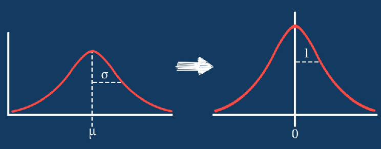
The usual standardization subtracts each feature’s mean and divides by its standard deviation:
Thus, z = 2 means that a value lies two standard deviations above the reference mean. The nonconstant columns in the fitting dataset acquire mean zero and variance one, provided the same variance convention is used throughout. StandardScaler uses the divisor n, equivalent to ddof=0.[1]
Normalization by a norm: transforming each observation
In another use of the term, normalization means dividing each nonzero observation vector by its norm. For the Euclidean norm:
This operation maps each row to unit length and preserves its direction, discarding the vector’s overall magnitude. It can be useful for text representations and comparisons using cosine similarity. It does not, by itself, put different columns on comparable scales; the norm must also be meaningful for the chosen representation.[3]
02 / ExampleUnits can change the nearest neighbor
Consider four fictional observations. Income is expressed in monetary units per month. We will use all four rows as the reference dataset to illustrate the transformations; we are not yet evaluating a predictive model.
| Observation | Age (years) | Monthly income |
|---|---|---|
| A | 20 | 2,000 |
| B | 22 | 3,000 |
| C | 40 | 2,100 |
| D | 50 | 5,000 |
Applying Euclidean distance directly to the original numbers gives a distance of approximately 1,000.002 from A to B, and 101.980 from A to C. C is closer to A despite a twenty-year age difference, because the difference in income dominates the calculation.
For min–max scaling, the age range is 30 and the income range is 3,000. For standardization, the means are 33 and 3,025; the standard deviations, calculated with divisor 4, are approximately 12.530 and 1,204.938.
| Row | Age min–max | Income min–max | Age z | Income z |
|---|---|---|---|---|
| A | 0.0000 | 0.0000 | −1.0375 | −0.8507 |
| B | 0.0667 | 0.3333 | −0.8779 | −0.0207 |
| C | 0.6667 | 0.0333 | 0.5587 | −0.7677 |
| D | 1.0000 | 1.0000 | 1.3567 | 1.6391 |
After min–max scaling, the distances from A to B and from A to C are:
≈ 0.3399 d′(A, C) = √[(20/30)² + (100/3,000)²]
≈ 0.6675 To D: d′(A, D) ≈ 1.4142. Among the other three observations, B is now the closest to A.
The nearest neighbor changed from C to B. The people and their original attributes did not change: the numerical comparison rule did. The example demonstrates sensitivity to scale; it does not establish that the second neighborhood is scientifically preferable. That requires justifying what “similar” means in the problem under study.
03 / FoundationsThree distinct reasons to scale
Geometry: deciding how proximity is measured
If each coordinate is transformed as x′j = (xj − bj)/sj, with sj > 0, the squared Euclidean distance between two observations becomes:
This identity shows that scaling introduces a weighting for each coordinate: every squared difference receives the factor 1/sj². This affects K-nearest neighbors when it uses a metric sensitive to scale, and K-means with its usual Euclidean objective. Standardization equalizes marginal variances in the fitting dataset; it does not equalize the information supplied by each variable or remove their correlations.[4]
Optimization: making the path to a solution easier
In problems fitted using gradient methods, very different scales can produce uneven curvature in the objective function. A learning rate small enough for one direction may make progress slow in another. Appropriate scaling can improve conditioning and help convergence, although it does not eliminate every numerical difficulty or guarantee a particular speedup.[5]
It is useful to distinguish the model from the algorithm used to fit it: the same family of models can be estimated through different numerical procedures. Consequently, “improves training” and “changes the statistical solution” are not equivalent claims.
Regularization: units also affect penalties
In a linear predictor, multiplying a feature by a constant allows its coefficient to be divided by that constant without changing its contribution to the prediction. An L1 or L2 penalty on the coefficients does change under this reparameterization if its form and strength remain fixed. This is why scale matters in Ridge, Lasso and regularized logistic regression.[6]
The rationale for scaling therefore extends beyond the explicit use of distances. In unpenalized least squares with an intercept and an invertible affine transformation of the features, the space of fitted predictions is preserved in exact arithmetic; numerical behavior may nevertheless change.
Choosing a scale means choosing how differences are compared.
04 / A particular casePCA: which variability do we want to preserve?
Principal component analysis seeks directions of maximum variance through linear combinations of the features. Working with centered data in their original units gives PCA of the covariance matrix; standardizing first, with a consistent variance convention, leads to PCA of the correlation matrix.
Differences in units can cause a feature with large numerical variance to dominate certain components. But a high mean does not imply high variance: a variable can have large values and vary very little. What matters for PCA is the spread and the structure of covariation.
Standardizing before PCA is an analytical decision. It may be justified when units are heterogeneous and the aim is to compare the features’ relative variation. If all features share units and their variance differences have substantive meaning, removing those differences may obscure relevant information.[4]
PCA should not be identified with gradient descent either. It is usually computed through singular value decomposition of the centered data or eigendecomposition of the covariance matrix. In scikit-learn, PCA centers the features but does not automatically standardize them.[7]
05 / JudgmentHow to choose a transformation
The starting point should be the model’s mechanism, the observed distribution and the meaning of the variables. The following options are working hypotheses to test, not guarantees of superiority:
| Situation | Option to evaluate | Caution |
|---|---|---|
| Comparing differences in units of spread | Standardization | The mean and standard deviation are sensitive to extremes. |
| Using a bounded reference interval | Min–max scaling | Future values may exceed the interval; extremes compress the remaining values. |
| Reducing the influence of extremes on scaling parameters | Median and interquartile range | Does not remove outliers or make the entire model robust. |
| Comparing vector direction or composition | Normalization by a norm | Discards overall magnitude. |
| Trees with splits on individual features | Keeping the original scale | Check the requirements of the other processing steps. |
Outliers and robust scaling
When a few extremes substantially affect the mean, standard deviation or range, a less sensitive reference is worth considering. A common transformation is:
RobustScaler applies this criterion by default. Here, “robust” refers to how the center and scale are estimated: an extreme observation can remain far away after transformation and still influence the subsequent estimator.[8]
Cases where scaling usually adds little
Conventional trees that split a feature using thresholds preserve, in exact arithmetic, the same possible partitions under affine transformations with positive slope. The ordering of values does not change. Scaling is therefore usually unnecessary for those trees and ensembles based exclusively on them; implementation or numerical precision differences may occur.[11]
A processing chain that includes distance-based selection, PCA or another step sensitive to scale may require scaling even when its final predictor is a tree. Evaluation should consider the entire procedure.
06 / ApplicationTransforming without leaking information
Scaling parameters are learned from data: means, standard deviations, extremes or quantiles. Computing them on the entire dataset before splitting training and test data allows the test set to influence model construction. This data leakage can produce an overly optimistic evaluation.
The operational rule is simple: fit the scaler only on training data and reuse its parameters on the other data. In cross-validation, fitting must be repeated on the training portion of each fold. A Pipeline allows this procedure to be carried out together with the estimator.[9]
from sklearn.datasets import load_iris
from sklearn.model_selection import (
    StratifiedKFold,
    cross_val_score,
    train_test_split,
)
from sklearn.neighbors import KNeighborsClassifier
from sklearn.pipeline import make_pipeline
from sklearn.preprocessing import StandardScaler

X, y = load_iris(return_X_y=True)
X_train, X_test, y_train, y_test = train_test_split(
    X, y, test_size=0.25,
    stratify=y, random_state=42,
)

model = make_pipeline(
    StandardScaler(),
    KNeighborsClassifier(n_neighbors=5),
)
cv = StratifiedKFold(
    n_splits=5, shuffle=True, random_state=42,
)

# The scaler is fitted within each fold.
scores = cross_val_score(
    model, X_train, y_train,
    cv=cv, scoring="accuracy",
)
print(f"Mean CV accuracy: {scores.mean():.3f}")

# Final fitting uses training data only.
model.fit(X_train, y_train)
print(f"Test accuracy: {model.score(X_test, y_test):.3f}")The example illustrates the proper separation between fitting and evaluation; it does not attempt to show that standardization always improves performance on Iris. For temporal data, observations grouped by person or other dependencies, the splitting strategy must also respect that structure.
When applying the model to future observations, the learned scaler is retained. Refitting it independently on each batch changes the input coordinates and breaks their correspondence with the trained model.
07 / ScopeWhat scaling does not resolve
Scaling is part of preprocessing, but it does not replace cleaning or data quality assessment. It does not correct measurement errors, duplicates, selection biases or incorrect labels; nor does it automatically impute missing values.
- Constant columns. If the range or standard deviation is zero, the corresponding formulas require specific handling. Such columns should be identified and a decision made about retaining them.
- Sparse data. Subtracting the mean can turn zeros into nonzero values and substantially increase memory use.
StandardScaler(with_mean=False)avoids centering when sparsity must be preserved.[1] - Categorical variables. Assigning numbers to categories does not automatically establish a legitimate order or distance. Their encoding requires a separate decision.
- Interpretation. A coefficient expressed per standard deviation answers a different question from one expressed per year or monetary unit. The chosen scale should be documented.
The decisive methodological question is which differences in the phenomenon we wish to preserve and which arise solely from its units of representation. Knowledge of the object of study guides that choice; validation allows its predictive consequences to be tested. Understood in this way, scaling is an explicit modeling decision.
08 / SourcesReferences and notes
Numbered citations refer to primary documentation for the tools and to university teaching material. The data and calculations in the age and income example were constructed for this article. Documentation consulted on October 26, 2026.
- Scikit-learn developers. (n.d.). StandardScaler. Scikit-learn documentation.
- Scikit-learn developers. (n.d.). MinMaxScaler. Scikit-learn documentation.
- Scikit-learn developers. (n.d.). Normalizer. Scikit-learn documentation.
- Scikit-learn developers. (n.d.). Importance of Feature Scaling. Scikit-learn examples.
- Scikit-learn developers. (n.d.). Stochastic Gradient Descent. Scikit-learn user guide.
- Scikit-learn developers. (n.d.). Linear Models. Scikit-learn user guide. See the sections on Ridge, Lasso and logistic regression.
- Scikit-learn developers. (n.d.). PCA. Scikit-learn documentation.
- Scikit-learn developers. (n.d.). RobustScaler. Scikit-learn documentation.
- Scikit-learn developers. (n.d.). Common pitfalls and recommended practices. Scikit-learn user guide.
- The Pennsylvania State University. (n.d.). SLR Model Assumptions. STAT 501: Regression Methods.
- Scikit-learn developers. (n.d.). Decision Trees. Scikit-learn user guide.
Leave a Comment/Deja un Comentario