
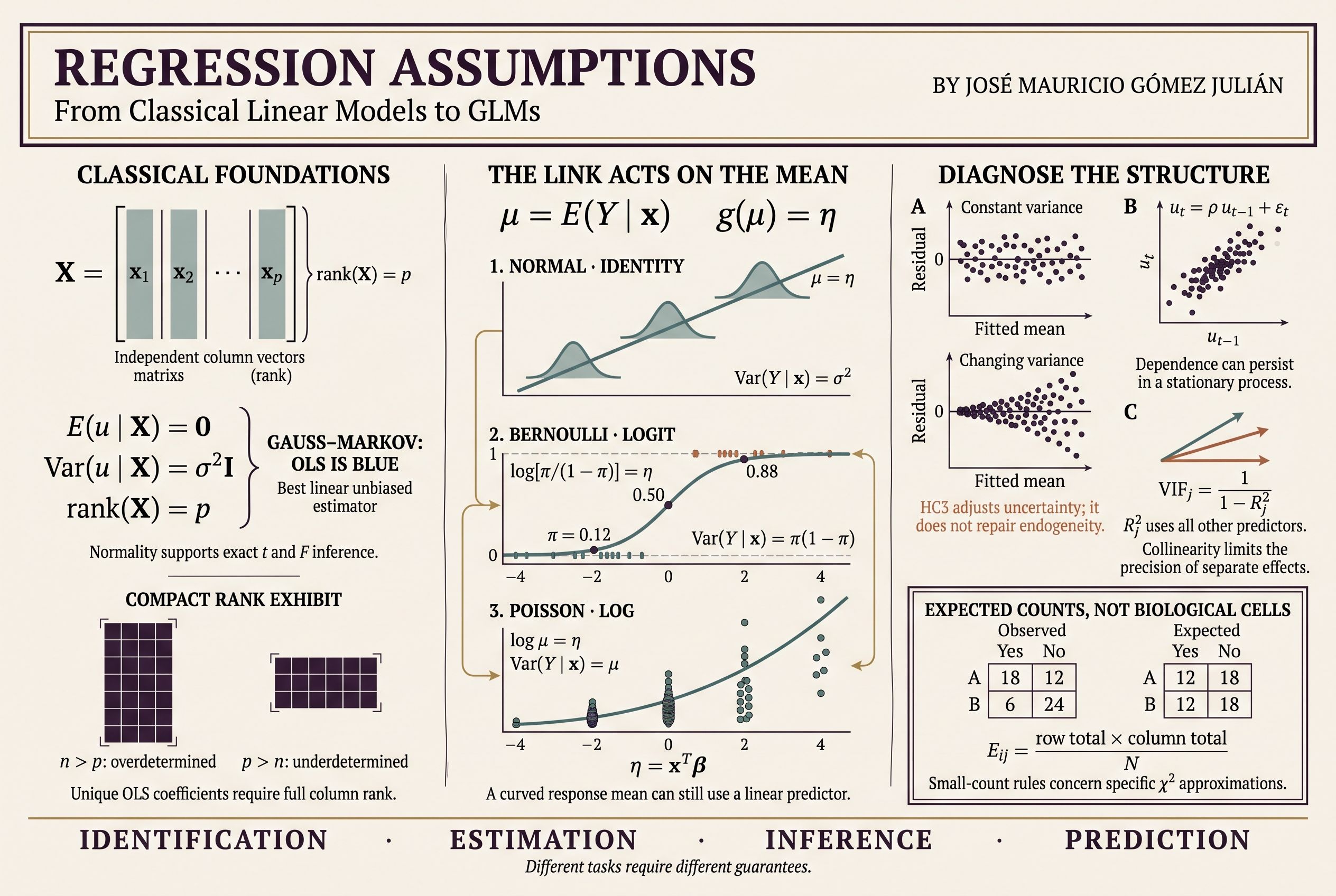
Marxist Philosophy of Science · Mathematical statistics
Assumptions of the Classical Linear Regression Model and Generalized Linear Models
Foundations, guarantees, diagnostics, and reproducible examples in R
01What models assume and what they allow us to conclude
A regression model connects a question about the world to a mathematical representation of a response distribution. Its assumptions establish the conditions under which particular conclusions are justified. Understanding them requires separating the existence of a fit, estimator properties, inferential validity, and predictive performance.
This article develops the classical linear regression model and generalized linear models (GLMs) through their geometric, algebraic, and probabilistic foundations. It connects practical diagnostics to a methodological qualification: no statistical procedure, by itself, turns an association into a causal explanation. Measurement, research design, and the historical and material conditions of the phenomenon remain part of the scientific problem.
A predictor may be continuous, categorical, or a transformation of another variable. Responses also have different forms. The task is to make the question, the support of the data, the mean function, and the uncertainty attributed to the process mutually coherent.
02From Galton to contemporary inference
Francis Galton used regression to study similarities in stature across generations. His 1886 papers, Regression towards mediocrity in hereditary stature and Family likeness in stature, preceded Natural Inheritance (1889). Here “mediocrity” refers to an average position rather than a judgment about people. The relevant phenomenon is that, after selecting parents with extreme heights, the average height of their offspring may be less extreme. [1]
Regression toward the mean does not require every offspring to move toward the average, nor is it a law of biological progress. For jointly normal standardized variables, the conditional mean is E(ZY|ZX=z)=ρz: when |ρ|<1, its magnitude is smaller than |z|. This identity illustrates the mechanism under that model; it does not automatically extend to every distribution.
Karl Pearson and Alice Lee extended the quantitative study of inheritance. Ronald A. Fisher developed tools for estimation, experimental design, and significance testing; Jerzy Neyman and Egon Pearson developed a testing framework concerned with repeated-sampling error control. Their methodological differences matter here more than personal anecdotes.
NHST stands for null hypothesis significance testing. Perezgonzalez critically examines common combinations of the Fisherian and Neyman–Pearson traditions. That interpretation should be attributed, and a p-value, a level α, and statistical power should be distinguished rather than treated as interchangeable. [2]
03Population, sample, and notation
A population distribution describes possible variation; a sample contains observed realizations. A parameter belongs to the population model; an estimator is a function of the sample; an estimate is its computed value. A statistic need not be a test statistic: a sample mean is also a statistic.
| Symbol | Meaning |
|---|---|
| n | Number of observations. |
| p | Total number of regression coefficients, including the intercept. |
| X, xiT | The n × p design matrix and its ith row. |
| β, β̂ | Population coefficient vector and its estimator. |
| ui, ûi | Unobserved disturbance and computed residual. |
| μi, ηi | Conditional mean and linear predictor. |
| σ², φ, Ω | Scalar variance, GLM dispersion, and error covariance matrix. |
X incorporates factor coding, powers, and interactions included in the specification. A categorical variable with several levels usually contributes several columns, so the number of original variables need not equal p. With an intercept, one column of X consists of ones.
04Model, loss, estimation, and algorithm
Regression models a characteristic of Y conditional on information X. For a linear conditional-mean model, the compact formulation is:
Y is the random response vector; Xβ represents its conditional mean under the specification; u contains deviations from that mean. Writing an equation does not automatically identify a causal mechanism. Disturbances may reflect individual variation, imperfect measurement, and omitted factors, but their relationship with X must be justified.
A loss criterion evaluates discrepancies. OLS minimizes the sum of squared residuals. Least absolute deviations minimizes the sum of their absolute values; in an unrestricted population problem, squared loss targets a conditional mean and absolute loss a conditional median. Under parametric restrictions, the result is the best approximation within the specified class.
Estimation can use least squares, maximum likelihood, moments, quasi-likelihood, or Bayesian methods. An algorithm, such as QR or a Newton iteration, computes the result. Different algorithms can solve the same criterion, and a model can be estimated using different criteria.
Connecting the extreme points, averaging pairwise slopes, or balancing the number of points above and below a line are possible geometric constructions, but they do not ensure identification, stability, or desirable statistical properties. Balancing signs alone does not uniquely determine a line. “Best fit” always requires a specified loss and constraints.
‖r‖∞ = maxi|ri|(02)
L2(r)=∑ri2=‖r‖22(03)
Here r is a residual vector and q is the norm order, distinct from the number p of coefficients. The 1/q root is part of the norm definition. The sum of squares is the squared Euclidean norm: it is not itself a norm, although both have the same minimizers. For 0<q<1, the corresponding expression generally fails the triangle inequality required of a norm.
Adding discrepancies presupposes appropriate comparability of units and weights. Independence is not required to define a norm; it may be required by the probability model used to justify an inferential procedure. Nor is every GLM discrepancy criterion a norm or a metric distance.
05What “linear” means
In simple regression, the intercept β0 is the mean’s height at x=0, provided that value belongs to the relevant domain. The slope β1 is the change in the mean per unit of x:
The general definition of a linear model concerns its coefficients. The following model describes a parabola and remains linear in β:
Its design columns are 1, x, and x². Log x, group indicators, and interactions are also admissible when the transformations are defined and the coefficients enter linearly. A function with an intercept is, strictly speaking, affine in the variables; statistical usage of “linear” includes that intercept.
By contrast, a mean β0+exp(β1x) is nonlinear in β1. Nonlinear least squares is a different optimization problem. The distinction concerns parametrization, not whether a plot looks curved.
The third situation illustrates why a small linear correlation can coexist with a strong curved association. A straight-line fit in the original variables may be inadequate, while a polynomial model, still linear in its parameters, captures the mean’s shape. Choosing additional terms requires theory and validation rather than inspecting in-sample fit alone.
06OLS: optimization, projection, and likelihood
The minimization problem
For each candidate b, compute predictions xiTb, subtract them from the observed values, and sum the squared differences. Squaring prevents sign cancellation and penalizes larger discrepancies more heavily. Differentiating ‖y−Xb‖² with respect to b gives −2XT(y−Xb). Setting it to zero yields the normal equations:
β̂ = (XTX)−1XTy(07)
The inverse expression requires full column rank: rank(X)=p. It is an analytical formula, not a programming recommendation. Numerically, QR and SVD avoid unnecessarily forming or inverting XTX, which worsens conditioning. [3]
The geometric interpretation
XTû = 0(08)
The fitted vector is the orthogonal projection of y onto the column space of X. H is the projection matrix and û=y−ŷ. Orthogonality XTû=0 follows from the OLS criterion: it does not demonstrate probabilistic independence or exogeneity. With an intercept, ∑ûi=0 as well.
For each observation, deviation from the mean splits into a fitted component and a residual. Squaring and summing eliminates the cross term by orthogonality. For unweighted OLS with an intercept, SST=∑(yi−ȳ)², SSR=∑(ŷi−ȳ)², and SSE=∑ûi². Abbreviations vary across texts; they are explicitly defined here.
SST>0 is required. R² summarizes in-sample fit; it does not establish causality, exogeneity, or predictive ability. Adding columns to nested models fitted to the same sample cannot increase SSE and therefore cannot decrease R². Adjusted R² penalizes degrees of freedom, but it does not replace external validation either.
When OLS coincides with maximum likelihood
If, conditional on X, errors are independent normal variables with common variance σ², the log-likelihood is:
− [1/(2σ2)] ∑i=1n(yi − xiTb)2(11)
For fixed positive σ², maximizing ℓ over b is equivalent to minimizing SSE: the remaining term is constant in b and the SSE multiplier is negative. Joint estimation of σ² retains the OLS solution for β when a regular maximum exists. In the normal model, its maximum-likelihood estimate is SSE/n, whereas SSE/(n−p) corrects bias in variance estimation. The distinction matters.
07Exogeneity: the meaning of zero conditional mean
Regressors may be treated as fixed in an experimental design or random when sampled jointly with the response. Conditioning on X allows both cases to share a framework, but fixed X does not, by itself, remove a misspecified error mean. The classical conditional unbiasedness argument requires E(u|X)=0.
This condition says that, given the complete design matrix, disturbances have no systematic mean deviation. It does not require every realized error to be zero or every subsample to have an exactly zero average. With random design, it implies E(u)=0 by iterated expectation and, under appropriate moment conditions, orthogonality to functions of X.
The first equality follows by substituting y=Xβ+u into the OLS formula. Conditional on X, the matrix multiplying u is fixed, so that term has zero expectation. The mean of β̂ over repeated samples therefore equals β. Neither homoskedasticity nor normality is needed in this argument.
Independence, covariance, and conditional mean
Independence of X and U, together with E(U)=0, implies E(U|X)=0. Zero covariance, however, implies neither independence nor zero conditional mean. The following counterexample makes the distinction explicit:
Cov(X,U)=0, E(U|X)=X2−1/3 ≠ 0(13)
Symmetry gives E(X)=E(X³)=0 and E(X²)=1/3, making the covariance zero. Yet U depends deterministically on X and its conditional expectation varies with X. A particular slope can sometimes be unbiased under weaker conditions; this does not make zero covariance and independence equivalent concepts.
How the condition can fail and how it is investigated
An omitted variable associated with X, simultaneous determination of response and predictors, certain measurement errors, or observation selection may produce endogeneity. The consequences depend on the specific structure. In time series, E(u|X)=0 conditions on the entire design and is generally stronger than a contemporaneous condition E(ut|xt)=0.
Residual plots can reveal incompatible functional forms; they cannot verify that every omitted influence is absent. Exogeneity rests on research design, timing, measurement, and theory. Instruments, experiments, and other identification strategies require further assumptions; changing standard errors does not resolve endogeneity.
08Gauss–Markov, precision, and inference
A conditional formulation of the theorem combines the following conditions, with σ² positive and finite:
Full rank provides a unique OLS coefficient vector. Zero conditional mean provides unbiasedness. The matrix σ²I combines homoskedasticity and zero covariances between distinct errors. Under these conditions, OLS is BLUE: the best linear unbiased estimator. “Linear” here describes the estimator’s dependence on Y, given X. [4]
Variance depends on both noise σ² and the information in X. Efficiency within the linear unbiased class does not ensure small standard errors: an uninformative design can leave substantial uncertainty even for the best estimator in that class.
Why the minimum property holds
Var(ÃY|X)−Var(AY|X)=σ2CCT ⪰ 0(16)
Any other conditionally unbiased linear estimator can be written as ÃY, where ÃX=I. Its difference from the OLS matrix is C, satisfying CX=0. Computing covariances eliminates the cross terms and leaves σ²CCT, a positive semidefinite matrix. For every linear combination of coefficients, this difference cannot reduce variance. That is the precise meaning of “best.”
Normality and exact tests
Joint conditional normality u|X∼N(0,σ²I) is not part of the preceding argument. Adding it, with n>p, gives the exact t and F distributions of the classical normal model:
SSE measures total residual variation; n−p subtracts the dimensions used to fit coefficients. The t-statistic’s numerator compares the estimate with the null value βj,0; its denominator expresses estimated uncertainty under the model. F-tests address joint linear restrictions. Changing the covariance structure changes the justification of these standard errors and tests.
Without normality, asymptotic inference may be available under moment, design, and dependence conditions supporting laws of large numbers and central limit theorems. A large n does not automatically repair endogeneity, nonidentification, dominant observations, or incorrectly handled dependence.
09Homoskedasticity and heteroskedasticity
Homoskedasticity requires Var(ui|X)=σ² for every observation. Variance is constant, not zero. Zero variance would eliminate conditional error variation and constitute a degenerate case. Heteroskedasticity allows variance to change across observations or with conditioning information.
Eight situations requiring interpretation
- Learning. Typing practice may reduce both the average number of mistakes and its variability. These are different characteristics: a mean trend does not establish heteroskedasticity.
- Economic scale. High-income households may exhibit greater dispersion in savings. The relevant quantity is savings variance conditional on income and the other predictors.
- Measurement quality. Institutions with different recording systems may have different precision. Measurement error in a predictor may also create endogeneity.
- Unusual observations. A large residual warrants examination but may arise from the same distribution. Response outliers, leverage, and influence are not synonyms.
- Omitted variables and mixtures. Combining groups with different means or variances can generate apparent patterns. Review the specification before attributing them to noise.
- Skewed predictors. Income concentration may affect design coverage and leverage. Skewness of X does not, by itself, imply changing conditional error variance.
- Transformations. Logs and other transformations can stabilize, preserve, or worsen dispersion; the outcome depends on the variation mechanism.
- Functional form. Fitting a straight line to a curved mean can produce residual structure. This is initially a mean-specification problem, not proof of genuine heteroskedasticity.
What remains and what is no longer guaranteed
Var(β̂|X)=BXTΩXB(18)
Ω denotes the conditional error covariance matrix. With heteroskedasticity alone and uncorrelated errors, it is diagonal. If E(u|X)=0 and the design has full rank, OLS remains linear and unbiased. Consistency requires further asymptotic conditions. The general BLUE guarantee and validity of the conventional formula s²(XTX)−1 are lost. Losing the guarantee does not prove inefficiency for every possible design.
Conventional standard errors can be too small or too large. Intervals and tests may therefore be distorted; there is no universal direction of inferential error.
Diagnosis and possible responses
Residual-versus-fitted and residual-versus-predictor plots help detect changes in dispersion. Tests such as Breusch–Pagan and White address specific hypotheses and may also react to misspecification. Failing to reject a test does not certify homoskedasticity.
V̂HC3=B[∑ixixiT ûi2/(1−hii)2]B(19)
This HC3 robust estimator uses hii, observation i’s leverage, to adjust its residual contribution. It preserves OLS coefficients and modifies the estimated covariance; it does not repair a wrong mean function or demonstrate exogeneity. Its justification is approximate and requires appropriate conditions, particularly concerning dependence and dominant observations.
β̂GLS=M−1XTΩ−1y(20)
If Ω is known, symmetric, and positive definite, generalized least squares incorporates its inverse as a weighting matrix. Diagonal Ω gives weighted least squares. Estimating Ω produces feasible GLS, whose performance depends on the variance model. Generalized least squares (GLS) must be distinguished from generalized linear models (GLMs).
What a logarithm actually does
The first-order approximation uses the derivative of log μ, which is 1/μ. If Y’s standard deviation is approximately proportional to its positive mean, dividing variance by μ² may stabilize it. If relative dispersion changes differently, the result may differ. A logarithm compresses high values of the transformed variable; transforming Y does not move points horizontally along X.
Y>0 must be respected, and changing scale changes the modeled quantity: E(log Y|X) generally differs from log E(Y|X). Exponentiating a prediction of log Y does not automatically estimate Y’s mean. Retransformation requires an appropriate distributional argument or correction. [5]
10Autocorrelation, dependence, and time
No autocorrelation requires Cov(ut,us|X)=0 for t≠s. With positive finite variances, this is equivalent to zero correlation, not independence in general distributions. A process can be random and possess memory. “Stochastic” therefore does not mean “without temporal structure.”
γ(h)=σε2ρ|h|/(1−ρ2)(22)
In this stationary AR(1) process, εt are independent innovations with zero mean and variance σ²ε. Covariance γ(h) depends on lag h. When ρ≠0, there is autocorrelation even though mean and variance do not change over time. Weak stationarity requires a constant mean and covariances depending on temporal separation rather than calendar date.
Mechanisms that can generate residual structure
- Persistence and inertia. Gradual adjustment after a recession, cycles, or persistent shocks can produce dependence if inadequately modeled.
- Excluded variables. An omitted factor evolving over time leaves a pattern in residuals. If related to the regressors, it may also create specification bias.
- Incorrect functional form. An omitted trend or seasonal component may resemble error dependence. Correcting the mean is distinct from changing its covariance.
- Economic cobweb. Agricultural supply may respond to previous prices because production takes time. This motivates dynamic equations without automatically establishing error autocorrelation in every specification.
- Lags. The past’s influence on the present calls for suitable variables and temporal structure. Including a lagged response changes exogeneity requirements.
- Aggregation and smoothing. Overlapping moving averages share observations and may induce dependence. Averaging disjoint blocks of independent errors need not do so.
- Differencing. Transformations change covariance structure. Even differencing white noise can introduce serial correlation.
- Nonstationarity. Stochastic trends may generate spurious regressions. Nonstationary variables can also be cointegrated, with a stationary combination; this requires a different analysis.
If εt is independent white noise, vt and vt−1 share εt−1 with opposite signs, explaining the negative covariance. This illustrates why a transformation cannot be judged merely by whether it smooths a plot.
Consequences and decisions
Under E(u|X)=0, OLS remains unbiased with nondiagonal covariances; consistency depends on further dependence and design conditions. In dynamic models, neither property should be assumed automatically. The general covariance of β̂ remains the expression involving Ω given earlier.
Conventional inference may fail, but there is no universal rule requiring every variance to be underestimated or R² always to be inflated. Spurious regression is a specific risk, distinct from any autocorrelation in a stationary series.
Inspect residuals in temporal order, their autocorrelation function, and model-appropriate diagnostics. Breusch–Godfrey tests specified forms of serial correlation; Durbin–Watson has a narrower scope. HAC estimates covariances robust to heteroskedasticity and temporal dependence under appropriate conditions; lag selection matters. Grouped data call for considering cluster-robust errors, with care when there are few groups. None of these corrections replaces an adequate temporal specification or causal identification strategy.
11Observations, rank, restrictions, and identification
Counting observations and coefficients is necessary but insufficient. If two columns of X are duplicates, increasing n does not identify their separate effects while duplication persists. Unique OLS coefficients require rank(X)=p.
| Dimensions | What follows |
|---|---|
| n>p | Overdetermined system. It may be consistent; OLS coefficients are unique if X has full column rank. |
| n=p | Invertible X gives unique interpolation. Residual degrees of freedom are zero. |
| n<p | Underdetermined system. X cannot have full column rank and unrestricted OLS coefficients are not unique. |
An exact solution to Xb=y exists if:
The augmented matrix [X|y] adds the response as a column. If rank increases, y lies outside the column space of X and there is no exact solution. Nevertheless, the least-squares problem has at least one minimizer. Coefficients may be nonunique under rank deficiency, but the fitted vector, as a projection onto that space, is unique.
An example with lines and observations
One observation (x1,y1) leaves infinitely many intercept-slope pairs. Two observations at distinct x values determine one line, but do not permit residual variance estimation with two free parameters. With at least three observations and nonconstant x, that variance can be estimated, although a minimal sample still offers very little precision.
Residual degrees of freedom count dimensions outside the fitted space. Imposing q independent compatible linear restrictions on an initially identifiable vector of p coefficients may reduce the free dimension to p−q and increase residual degrees of freedom to n−p+q. This must not be confused with reducing residual degrees of freedom.
Fixing a parameter at zero, such as a minimum diameter in a physical model, reduces free parameters only if it remains fixed during estimation. Its justification must come from the scientific problem, not the desire to obtain a solution. Restrictions can also identify initially rank-deficient problems, but must specifically eliminate the unidentified directions.
Pseudoinverse and regularization
The Moore–Penrose pseudoinverse selects the OLS minimizer with the smallest Euclidean norm. Selecting a solution does not establish that the data individually identified every coefficient. Values also depend on parametrization and measurement units.
Ridge penalizes slope coefficients; the intercept b0 remains unpenalized in this formulation. λ controls the fit-shrinkage trade-off. Standardizing predictors may be necessary to make penalties comparable. Regularization can improve prediction with many predictors, but changes the estimator and introduces bias; its strength is chosen within training, usually by validation.
12Overfitting, underfitting, and predictive error
Overfitting occurs when a procedure captures training-specific features that harm performance on new data from the relevant target. Underfitting occurs when the function class or fitting procedure fails to capture relevant relationships. Neither is synonymous with a particular algebraic configuration.
A model can underfit with many variables if it omits a crucial interaction or imposes the wrong functional form. It can also overfit with n>p, especially after extensive specification search. Underfitting should not be credited with strong generalization: both extremes can predict poorly.
The identity assumes Y0=f(x0)+ε0, with a new zero-conditional-mean error independent of training. The expectation on the left averages over training samples and new responses at x0. The first term is irreducible noise; the second is the square of E[f̂(x0)]−f(x0); the third measures how predictions vary across training samples. Bias can be zero: it is not inevitably positive.
Increasing flexibility often reduces approximation bias and increases variability in classical settings, but this is not a universal monotonic law for every algorithm. Modern models can exhibit more complicated behavior. Practical decisions require evaluating the complete procedure and its intended use. [6]
Training, validation, and testing
Fit parameters on training data, choose hyperparameters or specifications by validation, and reserve a final test set for evaluating the selected procedure. Model search is itself part of learning. Standardization, imputation, and feature selection must be learned within each split; doing them beforehand can leak information.
Time-series analysis preserves temporal ordering and uses appropriate cutoffs or windows. Grouped data may require splitting entire groups. A random split mixing dependent observations can measure an easier task than the real prediction problem.
13Multicollinearity, precision, and micronumerosity
No perfect multicollinearity requires linear independence of X’s columns. It does not require statistical independence of the variables. With an intercept, including every indicator for a categorical variable creates the dummy-variable trap: their sum reproduces the column of ones.
Under perfect collinearity, a nonzero direction c satisfies Xc=0. Consequently, β and β+c generate the same fitted mean and their coefficients cannot be separated without restrictions. A 0/0 formula in a simple case is a manifestation of nonidentification, not its general definition.
Factors that can reduce independent information
- Restricted design or coverage. Observing a narrow income range may leave little useful variation regardless of nominal sample size.
- Population structure. Income and dwelling size may be strongly related when explaining electricity consumption.
- Model construction. Powers and interactions can create highly correlated columns. Centering can improve parametrization without changing the fitted space.
- High dimensionality. If p>n, full column rank is impossible; this is an underdetermined, not overdetermined, configuration.
- Common trends. Predictors growing together may provide little separable variation and may require stationarity analysis in time series.
The variance inflation factor
Var(β̂j|X) = σ2 / [∑i(xij−x̄j)2(1−Rj2)](28)
Rj² comes from an auxiliary regression of predictor j on all remaining predictors, with an intercept in the usual formulation. The second expression concerns a slope under spherical errors. Full rank and nonzero variation in that column are required. With just two predictors, Rj² equals their squared correlation; with more columns, that substitution can be wrong. [7]
A VIF of 10 multiplies variance by 10 relative to the formula’s reference factor and standard error by √10, holding other components fixed. The threshold 10 is a guideline, not a universal validity boundary. Variables with several degrees of freedom require appropriate diagnostics, such as generalized VIFs.
Consequences
High but imperfect collinearity can increase uncertainty, coefficient sensitivity, and interval width while unbiasedness and BLUE remain under the other assumptions. A significant overall test, high R², and weak individual tests can coexist. Prediction within the observed region may be reasonable while extrapolation or separate attribution remains unstable.
Distinguishing systematic from erratic collinearity helps discuss variable structure and sampling or numerical limitations, but does not replace rank, conditioning, and precision. Goldberger used “micronumerosity” as a methodological parody: few observations and little independent variation also limit information. Salmerón Gómez and colleagues develop that connection. [8]
The views of Leamer, Achen, Blanchard, and Kennedy discussed by Gujarati and Porter share a warning: automatic remedies cannot manufacture information. That discussion is valuable when practical severity is related to the question and available data. Obtaining more informative observations, reformulating contrasts, or using substantive knowledge may be preferable to mechanically deleting a variable. Omitting a relevant confounder can introduce bias; ridge changes the inferential target. Efficiency, precision, and computational stability are related but distinct dimensions. [9]
14The three components of a generalized linear model
A GLM combines a conditional response distribution, a linear predictor, and a link function. “Generalized” does not mean assumption-free: it broadens the permitted distributions and mean relationships while retaining an explicit structure. The normal linear model with identity link is one case.
μi is Yi‘s mean given its predictor information; ηi adds specified effects on the link scale. The link transforms the conditional mean. It need not be applied to each observed response. This distinction accommodates Poisson zeros and logistic 0/1 responses without computing log 0 or logit 0 on the data. [10]
Distribution and exponential family
This form covers densities or probability mass functions relative to an appropriate measure. θi is the canonical parameter; b determines moments; ai incorporates dispersion and known weights; c normalizes the distribution. Under exponential-family regularity conditions:
The last equality uses ai(φ)=φ/wi, with known wi>0. In unweighted cases wi=1. For binomial proportions, the number of trials plays this role. The variance form is not chosen arbitrarily after fitting the mean.
| Model | Response and mean | Illustrative link | Variance |
|---|---|---|---|
| Normal | Continuous; μ∈ℝ | g(μ)=μ | σ² |
| Bernoulli | Y∈{0,1}; μ=π | log[π/(1−π)] | π(1−π) |
| Binomial count | Y∈{0,…,m}; μ=mπ | logit(μ/m) | mπ(1−π) |
| Poisson | Nonnegative count; μ>0 | log μ | μ |
| Gamma | Positive continuous; μ>0 | log μ, among others | φμ² |
Gamma also admits an inverse link; the log link shown is a common option rather than its canonical link. The exponential distribution is a Gamma case. The multinomial can be incorporated through extensions with a vector response and multiple linear predictors; it should not be inserted into a scalar formula without that qualification. [11]
Logistic and Poisson regression
In logistic regression, πi is the success probability. The logit link allows unrestricted real η and returns probabilities between zero and one. exp(βj) expresses an odds ratio for a unit increase in predictor j, holding other terms fixed and respecting interactions; it is not automatically a risk ratio.
In Poisson regression, exp(βj) multiplies the mean for a unit change, subject to the same qualification about interactions. Variance equals the conditional mean: changes with X are part of the model. An overall sample variance greater than the overall sample mean does not establish conditional overdispersion.
When observations have different positive exposures ti, such as follow-up times, log ti enters as an offset with coefficient fixed at one. Then exp(xiTβ) models a rate. Comparing counts without exposure can confuse duration with intensity.
Independence and conditional structure
In the basic independent GLM, responses are independent conditional on the design and parameters. Shared subjects, schools, households, or repeated measurements may violate this structure. Exchangeability means invariance under permutations and permits dependence: it cannot simply replace independence. Generalized mixed models and generalized estimating equations address other structures with different targets.
Predictors need not all share the same scale, nor must deviations be independent of the mean. Coherent measurement and a correctly specified conditional distribution are required for the corresponding likelihood inference. In a GLM, deviation magnitudes can change with μ according to V(μ).
15GLM estimation, dispersion, and goodness of fit
Maximum likelihood and its conditions
With conditionally independent responses, the likelihood multiplies their distributions and the log-likelihood adds contributions. Coefficients maximize that sum under the chosen link and family. Maximum likelihood does not require a large sample to be defined; many approximations for its standard errors and tests are asymptotic.
A finite maximum need not exist. In logistic regression, complete or quasi-complete separation may send coefficients toward infinity; an algorithm may issue warnings or return very large values. Full rank alone does not exclude this problem. Diagnosis and, depending on the target, penalized or other specifically justified procedures are required.
Iteratively reweighted least squares
Wii=(dμi/dηi)2/Var(Yi|xi)(35)
At iteration m, compute means μ, derivatives dμ/dη, a working response z, and weights W. Then solve a weighted problem on the predictor scale. These expressions assume no offset; an offset requires incorporating the corresponding known term. Matrices must have appropriate rank, and derivatives and variances must permit the computation.
IRLS does not turn every GLM into OLS on a fixed transformation of the data: z and W are updated. For the normal model with identity link and common variance, the update recovers least squares. R’s glm() uses this type of procedure by default. [12]
Deviance and model comparison
ℓsat is the saturated model’s log-likelihood, fitting one mean per observation; ℓfit belongs to the model being assessed. The comparison uses the same dispersion where appropriate. D* denotes scaled deviance and D unscaled deviance under the convention used here. Sources vary in terminology: check the definition rather than the label alone.
For a normal model with dispersion σ², D=SSE and D*=SSE/σ². In Poisson regression, φ=1 and both coincide:
The convention for y=0 follows from the limit of y log y. No arbitrary modification of zeros is required to compute this discrepancy. Its expression depends on the distribution and is not merely a Euclidean norm. The saturated model is a discrepancy benchmark, not a predictive recommendation.
This Pearson expression applies to unweighted responses with Var(Y|X)=φV(μ). In Poisson regression, V(μ)=μ. With n>p, the ratio may serve as an approximate dispersion estimator or diagnostic, depending on the model. A high value may reflect overdispersion, dependence, influential data, or an incorrect mean; it does not identify the cause on its own.
A strict Poisson GLM fixes φ=1. Overdispersion relative to that model must be addressed: quasi-Poisson allows Var(Y|X)=φμ; negative binomial introduces another mean-variance relationship; mixed models can represent shared heterogeneity. These alternatives have different assumptions. For individual Bernoulli responses, variance is determined by probability; a free scale requires careful interpretation of the variation or grouping mechanism.
The likelihood-ratio approximation requires nested models, the same response and sample, identifiability, and regularity, including interior parameter values and appropriate asymptotic conditions. q is the dimension difference. Boundaries, separation, and sparse data may invalidate the usual reference distribution. AIC counts k estimated parameters, including dispersion parameters where applicable, and compares comparable likelihoods.
Quasi-families need not specify a full likelihood; ordinary AIC and likelihood-ratio testing cannot simply be used as if they did. Nor is D≈χ² a universal rule for every distribution, individual-observation setup, and sample size. Absolute goodness of fit must be distinguished from comparisons between nested models.
16Expected frequencies: what a cell means
In contingency tables, cell means a table entry. Recommendations about small expected counts concern the quality of particular chi-squared approximations. They do not concern biological cells or require every sampling unit to contain five observations. Nor are they universal assumptions of all GLMs.
Consider this illustrative table, which does not represent an actual study:
| Group | Outcome yes | Outcome no | Total |
|---|---|---|---|
| A | 18 | 12 | 30 |
| B | 6 | 24 | 30 |
| Total | 24 | 36 | 60 |
Under row-column independence, joint probability factorizes. Multiplying by N and estimating marginal probabilities gives Eij. The first expected count is 30×24/60=12; the second is 30×36/60=18. Expectations are 12,18 in both rows. They differ from observed counts 18,12 and 6,24.
The Pearson sum is 10; with one degree of freedom and no continuity correction, its chi-squared reference gives approximately p=0.001565. This illustrates the computation rather than supporting a substantive claim about real groups.
A classical guideline for certain tables avoids expected counts below 1 and a large proportion—often 20%—of cells with expected counts below 5. This is a contextual heuristic, not an exact mathematical boundary. Its relevance depends on the sampling scheme, dimensions, frequency distribution, and statistic. [13]
When the approximation is poor, appropriate exact or simulation methods may be considered. Fisher’s exact test for a 2×2 table uses a conditional distribution with fixed margins; it is not an automatic substitute for every table or design. Merging categories requires substantive justification and changes the question. Paired or grouped observations need procedures respecting their dependence.
17From assumptions to practical diagnostics
Useful diagnosis starts with the question and design. Auxiliary tests provide partial evidence rather than global validity certificates. Before selecting a remedy, determine whether the issue concerns the mean, variance, dependence, identification, or predictive task.
| Aspect | Evidence to examine | Possible response |
|---|---|---|
| Mean and link | Residuals, scientific knowledge, patterns by group. | Respecify terms, interactions, or link and validate. |
| Variance | Conditional dispersion, standardized residuals, specific tests. | HC errors, justified weights, or an appropriate family/variance. |
| Dependence | Time order, ACF, repeated units, group structure. | Dynamics, HAC, clustering, mixed models, or GEE as appropriate. |
| Rank and collinearity | Redundant columns, QR/SVD, VIF, conditioning. | Reparametrize, obtain information, or impose justified restrictions. |
| Influence | Leverage, studentized residuals, Cook’s distance. | Check records and perform sensitivity analysis. |
| Generalization | Out-of-sample error and stability across periods or groups. | Task-appropriate validation and selection within training. |
| Causal identification | Design, confounders, selection, timing. | An explicit causal argument and identification strategy. |
Residuals are not the original errors
Even under spherical errors, fitted residuals are neither independent nor identically variable: estimating coefficients by projection introduces covariances and makes residual variance depend on leverage. This motivates standardization and avoids demanding that residuals literally possess every property assumed for u.
A Q–Q plot examines distributional compatibility and can reveal tails or outliers, but interpretation must consider sample size, leverage, and structure. Nonnormal marginal Y or X does not, by itself, violate conditional error normality. Nor is normal Y required for logistic or Poisson regression.
A high-leverage observation has unusual predictor values; a large-residual observation differs from its prediction; an influential observation substantially changes the fit when removed. Observations should not be deleted merely because they inconvenience a model. Investigate their origin and report sensitivity while preserving the scientific question.
18A reproducible R laboratory
The following ten experiments use only base R and the stats package distributed with R. Every block is independent, sets a seed when generating randomness, and uses simulated data or an illustrative table. Known population coefficients help clarify what each procedure computes. The checks verify mathematical identities; they do not certify a real study’s validity.
A. A curve that remains a linear model
A quadratic mean is simulated and compared using a straight line, a polynomial linear in coefficients, and its equivalent normal GLM. Increasing R² concerns in-sample fit; coefficient equality checks the normal-identity equivalence of lm() and glm().
set.seed(240901)
n <- 180
x <- runif(n, -2, 2)
y <- 1 + 0.8*x + 0.6*x^2 + rnorm(n, sd = 0.7)
dat <- data.frame(x, y)
line <- lm(y ~ x, data = dat)
curve <- lm(y ~ x + I(x^2), data = dat)
normal_glm <- glm(y ~ x + I(x^2), data = dat,
                  family = gaussian(link = "identity"))
stopifnot(max(abs(coef(curve)-coef(normal_glm))) < 1e-8)
print(round(coef(curve), 4))
print(c(line_R2 = summary(line)$r.squared,
        curve_R2 = summary(curve)$r.squared,
        df = df.residual(curve)))
par(mfrow = c(1, 2))
plot(fitted(line), resid(line), main = "Linear mean")
abline(h = 0, lty = 2)
plot(fitted(curve), resid(curve), main = "Quadratic mean")
abline(h = 0, lty = 2)
par(mfrow = c(1, 1))
B. Heteroskedasticity and HC3 covariance
Standard deviation increases with x. Calculating HC3 preserves the OLS coefficients. The second fit’s weights use the known generating variance: this demonstrates correct weighting in simulation rather than a procedure that automatically knows the variance in real data.
set.seed(240902)
n <- 220
x <- runif(n, 0, 4)
sigma <- 0.25 + 0.65*x
y <- 2 + 1.5*x + rnorm(n, sd = sigma)
fit <- lm(y ~ x)
X <- model.matrix(fit)
h <- hatvalues(fit)
stopifnot(fit$rank == ncol(X), all(h < 1))
# A maps y to OLS coefficients; QR avoids inverting X'X.
A <- qr.coef(qr(X), diag(n))
B <- sweep(A, 2, resid(fit)/(1-h), FUN = "*")
V_HC3 <- tcrossprod(B)
weighted <- lm(y ~ x, weights = 1/sigma^2)
print(cbind(estimate = coef(fit),
            conventional_SE = sqrt(diag(vcov(fit))),
            HC3_SE = sqrt(diag(V_HC3))))
print(coef(weighted))
stopifnot(all(eigen(V_HC3, symmetric=TRUE)$values > 0))
C. Residuals with memory
Predictors are generated independently of an AR(1) error. The residual ACF reveals persistence. The block illustrates diagnosis; temporal inference additionally requires an appropriate covariance estimator or specification.
set.seed(240903)
n <- 240
x <- rnorm(n)
u <- as.numeric(arima.sim(model = list(ar = 0.7), n = n))
y <- 1 + 0.8*x + u
fit <- lm(y ~ x)
acf1 <- acf(resid(fit), plot = FALSE)$acf[2]
print(c(residual_lag1_ACF = acf1))
par(mfrow = c(1, 2))
plot(resid(fit), type="l", xlab="Time", ylab="Residual")
acf(resid(fit), main="Residual ACF")
par(mfrow = c(1, 1))
# This is a dependence diagnostic, not a HAC correction.
D. A redundant column and degrees of freedom
The third column duplicates an existing direction. R reports a nonestimable coefficient, while rank determines the correct residual degrees of freedom. The second fit interpolates two points, leaving zero residual degrees of freedom.
x <- 1:6
y <- c(2.1, 2.9, 4.2, 4.8, 6.1, 7.2)
X <- cbind(intercept=1, x=x, double_x=2*x)
fit <- lm(y ~ x + I(2*x))
print(c(n=nrow(X), p=ncol(X), rank=qr(X)$rank,
        residual_df=df.residual(fit)))
print(coef(fit))
stopifnot(fit$rank == 2, df.residual(fit) == 4,
          anyNA(coef(fit)))
# Two observations, two coefficients: interpolation, no residual df.
saturated <- lm(c(2, 5) ~ c(0, 1))
print(c(residual_df=df.residual(saturated)))
stopifnot(df.residual(saturated) == 0)
E. VIF using every remaining predictor
The auxiliary regression uses the remaining predictor set rather than just a pairwise correlation. VIFs and a condition number are shown; the latter also depends on units and parametrization.
set.seed(240904)
n <- 250
x1 <- rnorm(n)
x2 <- 0.98*x1 + 0.15*rnorm(n)
x3 <- rnorm(n)
Z <- data.frame(x1, x2, x3)
vif <- sapply(names(Z), function(target) {
  aux <- lm(reformulate(setdiff(names(Z), target),
                        response=target), data=Z)
  1/(1-summary(aux)$r.squared)
})
print(round(vif, 3))
print(c(condition_number=kappa(model.matrix(~., Z), exact=TRUE)))
stopifnot(all(vif >= 1), vif["x1"] > 10, vif["x3"] < 2)
F. Probabilities and intervals in logistic regression
Approximate inference is constructed on the link scale and transformed using the inverse logit. Intervals concern conditional probabilities rather than predictions of an individual binary response. exp(β̂) gives odds ratios in this specification without interactions.
set.seed(240905)
n <- 400
x <- rnorm(n)
prob <- plogis(-0.4 + 1.1*x)
y <- rbinom(n, size=1, prob=prob)
fit <- glm(y ~ x, family=binomial(link="logit"))
new <- data.frame(x=c(-1, 0, 1))
pred <- predict(fit, newdata=new, type="link", se.fit=TRUE)
z <- qnorm(0.975)
result <- data.frame(x=new$x, probability=plogis(pred$fit),
  lower=plogis(pred$fit-z*pred$se.fit),
  upper=plogis(pred$fit+z*pred$se.fit))
print(round(result, 4))
print(exp(coef(fit)))
stopifnot(fit$converged, all(result$probability > 0),
          all(result$probability < 1))
# Intervals target conditional probabilities, not new 0/1 outcomes.
G. Counts, exposure, and quasi-Poisson
Doubling exposure at fixed x doubles the mean count rather than the rate. The Pearson ratio is diagnostic. With the same link and data, Poisson and quasi-Poisson give the same coefficients here but treat dispersion differently; ordinary AIC is undefined for the quasi-family.
set.seed(240906)
n <- 320
x <- rnorm(n)
exposure <- runif(n, 0.5, 3)
mu <- exposure*exp(0.2 + 0.5*x)
y <- rpois(n, lambda=mu)
dat <- data.frame(y, x, exposure)
fit <- glm(y ~ x + offset(log(exposure)), data=dat,
           family=poisson(link="log"))
quasi <- glm(y ~ x + offset(log(exposure)), data=dat,
             family=quasipoisson(link="log"))
phi <- sum(residuals(fit, type="pearson")^2)/df.residual(fit)
print(c(Pearson_dispersion=phi, Poisson_AIC=AIC(fit),
        quasi_AIC=AIC(quasi)))
new <- data.frame(x=c(0, 0), exposure=c(1, 2))
means <- predict(fit, newdata=new, type="response")
print(means)
stopifnot(fit$converged,
  max(abs(coef(fit)-coef(quasi))) < 1e-7,
  abs(means[2]/means[1]-2) < 1e-8, is.na(AIC(quasi)))
H. A positive response with Gamma
The simulation has mean exp(0.7+0.6x), Gamma shape 4, and dispersion 1/4. Both mean and dispersion are estimated. Exact recovery of every population value is not expected in a finite sample.
set.seed(240907)
n <- 260
x <- runif(n, -1, 1)
mu <- exp(0.7 + 0.6*x)
y <- rgamma(n, shape=4, scale=mu/4)
fit <- glm(y ~ x, family=Gamma(link="log"))
print(round(coef(fit), 4))
print(c(estimated_dispersion=summary(fit)$dispersion))
stopifnot(fit$converged, all(fitted(fit) > 0))
I. Observed counts, expected counts, and two inferential references
Compute expected counts under independence, reproduce X²=10, and show Fisher’s test to distinguish an asymptotic reference from an exact conditional one. No continuity correction is used for the example’s Pearson test.
observed <- matrix(c(18,12,6,24), nrow=2, byrow=TRUE,
  dimnames=list(group=c("A","B"), outcome=c("yes","no")))
expected <- outer(rowSums(observed), colSums(observed))/sum(observed)
pearson <- chisq.test(observed, correct=FALSE)
print(expected)
print(c(X2=unname(pearson$statistic), p=pearson$p.value,
        fraction_expected_below5=mean(expected < 5)))
print(fisher.test(observed))
stopifnot(all(expected == pearson$expected),
          abs(unname(pearson$statistic)-10) < 1e-10)
J. Fitting and validation tell different stories
Degrees 1, 3, and 12 are compared for a cubic mean. Training error cannot increase as these nested spaces expand, but performance on new data may deteriorate. The simulation illustrates one outcome rather than proving a universal performance ordering. If this validation set selects the degree, a separate final test is required for performance reporting.
set.seed(240908)
signal <- function(x) 0.8 + 0.7*x - 0.5*x^2 + 0.6*x^3
train <- data.frame(x=runif(45, -1.5, 1.5))
train$y <- signal(train$x) + rnorm(nrow(train), sd=0.5)
validation <- data.frame(x=runif(1200, -1.5, 1.5))
validation$y <- signal(validation$x) + rnorm(nrow(validation), sd=0.5)
results <- do.call(rbind, lapply(c(1,3,12), function(d) {
  fit <- lm(y ~ poly(x, degree=d), data=train)
  data.frame(degree=d,
    train_MSE=mean(resid(fit)^2),
    validation_MSE=mean((validation$y-predict(fit, validation))^2))
}))
print(results)
stopifnot(all(is.finite(as.matrix(results))),
  all(diff(results$train_MSE) <= 1e-10))
# Choose on validation; assess the selected procedure on a fresh test set.
Check values from the execution
The stated seeds and R 4.3.3 produced the following rounded values. These help identify each block’s output rather than demand exact recovery of population parameters in a finite sample.
| Example | Result |
|---|---|
| Quadratic normal | β̂ ≈ (1.0072; 0.8449; 0.5637). |
| Heteroskedastic slope | Conventional SE ≈ 0.09744; HC3 ≈ 0.11037. |
| VIF | 43.469; 43.475; 1.002. |
| Poisson | Pearson dispersion ≈ 1.00086. |
| 2×2 table | X²=10; p≈0.0015654 without continuity correction. |
| Validation, degrees 1 / 3 / 12 | MSE ≈ 0.4951 / 0.2722 / 0.4042. |
19What each condition guarantees: an operational synthesis
| Condition | Guarantee or role | Does not establish |
|---|---|---|
| rank(X)=p | Unique OLS coefficients. | Exogeneity or generalization. |
| E(u|X)=0 and full rank | Conditional OLS unbiasedness. | Efficiency without covariance conditions. |
| Var(u|X)=σ²I and preceding conditions | The OLS BLUE property. | High precision for every design. |
| Joint conditional normality and n>p | Exact t/F inference under the rest of the normal model. | Causality or correct specification. |
| GLM family, link, and conditional structure | A mean-and-variation model compatible with the support. | Automatic existence of a finite maximum. |
| Inferential regularity and informative data | Justifiable asymptotic approximations. | A universal count or sample-size rule. |
| Validation matching intended use | Predictive evidence for the task evaluated. | Guaranteed transfer to another population. |
A model provides a mathematical mediation between measurements and scientific questions. A distribution or parameter does not replace the phenomenon: it selects aspects of its variation under stated conditions. Economic accumulation, institutional organization, or a process’s historicity can guide specification, but must connect to observable mechanisms and a design supporting the inferences.
Estimating a relationship, quantifying its uncertainty, predicting, and explaining causally are related tasks requiring different justifications.
A responsible report specifies the response and scale, design and sample, mean function, distribution or covariance, estimator, diagnostics, uncertainty, and scope of generalization. A multidimensional evaluation keeps these dimensions connected rather than reducing validity to a single p-value or a high R².
20A glossary of essential distinctions
- Error / residual
- Deviation from the population model / difference from the computed fit.
- Unbiasedness / consistency
- An expectation property under repeated sampling / convergence toward the target as information grows under a specified asymptotic regime.
- Efficiency / precision
- Variance comparison within a class / the actual magnitude of uncertainty.
- Independence / uncorrelatedness
- Factorization of the joint distribution / zero covariance when defined; the latter does not imply the former.
- Linearity / straightness
- Linear dependence on coefficients / the geometric shape of a plot in selected variables.
- Link / response transformation
- A function applied to the conditional mean / a function applied to an observed value; their targets are not generally equivalent.
- Overdetermination / overfitting
- More equations than unknowns / training adaptation that harms relevant prediction.
- Parameter / statistic
- A population-model characteristic / a function computed from observations, including but not limited to a test statistic.
- GLM / GLS
- Generalized linear model / generalized least squares; a probability-model family and an estimation method are not synonyms.
- Cell / sampling unit
- An entry in a frequency table / an element selected under the sampling design.
21References and sources
The following references support the revised exposition. Figures are original educational reconstructions and simulations rather than reproductions of plates from Greene or Gujarati and Porter.
- Galton, F. (1886). Regression towards mediocrity in hereditary stature. Journal of the Anthropological Institute, 15, 246–263. View source.
- Perezgonzalez, J. D. (2015). Fisher, Neyman–Pearson or NHST? A tutorial for teaching data testing. Frontiers in Psychology, 6, 223. View source.
- University of Illinois Urbana–Champaign, CS 357. Least Squares Fitting. View source.
- Taboga, M. (2021). Gauss Markov theorem. Lectures on Probability Theory and Mathematical Statistics. View source.
- NIST/SEMATECH. Transformations to Improve Fit and Equalize Variances. e-Handbook of Statistical Methods, §4.6.2.4. View source.
- James, G., Witten, D., Hastie, T., & Tibshirani, R. (2021). An Introduction to Statistical Learning, with Applications in R. 2nd ed. Springer. View source.
- Penn State University, STAT 462. 10.7 — Detecting Multicollinearity Using Variance Inflation Factors. View source.
- Salmerón Gómez, R., Blanco Izquierdo, V., & García García, C. (2016). Micronumerosidad aproximada y regresión lineal múltiple. Anales de ASEPUMA, 24, 1–17. View source.
- Gujarati, D. N., & Porter, D. C. (2010). Econometría. 5th ed. McGraw-Hill.
- McCullagh, P. (1992). Introduction to Nelder and Wedderburn (1972): Generalized Linear Models. In Breakthroughs in Statistics, vol. II, 543–546. View source.
- R Core Team. Family Objects for Models. Documentation for stats::family. View source.
- R Core Team. Fitting Generalized Linear Models. Documentation for stats::glm. View source.
- Penn State University, STAT 504. Advanced Topics II: sparse tables and chi-squared approximations. View source.
- Greene, W. H. (2012). Econometric Analysis. 7th ed. Pearson.
- McCullagh, P., & Nelder, J. A. (1989). Generalized Linear Models. 2nd ed. Chapman & Hall.
- JOSÉ MAURICIO GÓMEZ JULIÁN (2021; originally published as Isadore Nabi). Supuestos del modelo clásico de regresión lineal y de los modelos lineales generalizados. View source.
- MIT CSAIL. Solving over- and under-determined sets of equations. View source.
- Penn State University, STAT 462. 12.4 — Generalized Linear Models. View source.
- R Core Team. Predict Method for GLM Fits. View source.
Supplementary sources retained from the 2021 article
Retained for bibliographic traceability. Forums and popular explanations do not replace the definitions and mathematical conditions developed above. Some historical links may have changed.
- Banerjee, A. (2019). Intuition behind model fitting: Overfitting v/s Underfitting.
- Bhuptani, R. (2020). What is the difference between linear regression and least squares? Quora.
- Cross Validated (2018). Will log transformation always mitigate heteroskedasticity?
- Guanga, A. (2018). Machine Learning: Bias VS. Variance.
- Nabi, I. (2021). Modelos lineales generalizados.
- Penn State University, STAT 462. 10.4 — Multicollinearity.
- Penn State University, STAT 504. Introduction to Generalized Linear Models. Link cited in 2021.
- ResearchGate (2014). How it can be possible to fit the four-parameter Fedlund model by only 3 PSD points?
- ResearchGate (2019). Is there a rule for how many parameters I can fit to a model, depending on the number of data points I use for the fitting?
- Simon Fraser University (2011). The Classical Model.
- Cross Validated (2017). “Least Squares” and “Linear Regression”, are they synonyms?
- Wikipedia (2021). Overdetermined system.
- Zhao, J. (2017). More features than data points in linear regression?
Leave a Comment/Deja un Comentario