
Marxist Philosophy of Science · Mathematical statistics
The Kruskal–Wallis Test: Foundations, Assumptions, Calculation, and Interpretation in R
From pooled ranks to defensible inference: ties, Dunn comparisons, Holm adjustment, and effect size.
01. Overview and method selection
Comparing several groups requires deciding which difference matters: a difference in means, location, spread, or distributional structure. The Kruskal–Wallis test addresses part of this problem through the ordering of observations. Its appeal lies in constructing a test that does not require a normal response distribution, while retaining explicit assumptions.
Kruskal and Wallis (1952) developed a procedure for independent samples based on ranks in the pooled data. Calling it a “nonparametric one-way ANOVA” is useful provided that replacing values with ranks also changes the information used and the interpretation of the test. Although usually applied to three or more groups, it can also be computed for two. Its relationship to Wilcoxon–Mann–Whitney in that case does not mean that every approximation and correction produces exactly the same p-value.
| Situation | Procedure to consider | Necessary qualification |
|---|---|---|
| Means; independent groups; approximately normal errors and a common variance | Classical one-way ANOVA | Normality concerns within-group errors, rather than the distribution obtained by pooling every observation. |
| Means; independent groups; approximately normal errors and different variances | Welch ANOVA | A common variance is unnecessary; severe skewness, dependence, and influential values still require attention. |
| A rank-based comparison; independent groups | Kruskal–Wallis | A specific location or median interpretation requires comparable distributional shapes and spreads. |
| The same subjects in every condition; complete blocks with one observation per cell | Friedman, when the design permits | Repeated measurements cannot be treated as independent observations. |
| A conditional median is the direct target, or covariates or a hierarchy are present | Quantile regression or models appropriate to the design | Define the target and dependence structure; these models are outside the scope of this article. |
The official documentation distinguishes these procedures: oneway.test(..., var.equal = FALSE) applies Welch, kruskal.test() uses ranks, and friedman.test() addresses unreplicated complete block designs (R Core Team, n.d.-b, n.d.-c, n.d.-d). Avoid turning a sequence of normality and variance tests into an automatic method selector: define the question and examine the design first.
02. Hypotheses and interpretation
Let X1, …, Xk be the population responses, with distribution functions Fi. A general formulation of the null hypothesis is:
The general alternative allows at least one distribution to differ. However, Kruskal–Wallis is not a universal detector of every distributional difference: its statistic summarizes differences in mean ranks. Some alternatives, including certain symmetric differences in spread, can leave these mean ranks approximately equal and yield low power.
A specific location interpretation can be supported by a shift model:
In this model, every group shares a distributional shape and spread, and only θi changes. Testing identical distributions then amounts to testing equal locations; if the median is unique, it also amounts to testing equal medians. Outside that framework, equal medians are insufficient to establish the null, and rejecting the null does not establish different medians.
The NIST manual states the null in terms of identical populations, whereas the R documentation describes location parameters. These accounts connect through an explicitly stated shift model, rather than an unstated assumption (National Institute of Standards and Technology [NIST], n.d.; R Core Team, n.d.-c).
Describing data with medians does not turn a rank test into a test exclusively about medians.
03. Assumptions and design
| Aspect | What needs justification | What is insufficient |
|---|---|---|
| Independence | Each unit contributes an independent observation, and groups are mutually independent. | Equal sample sizes or successful software execution. |
| Sampling or assignment | How units were selected and which population is the target of generalization. | A small p-value does not correct a biased sample. |
| Measurement scale | Responses have a coherent ordering, with comparable measurement across groups. | Arbitrary numerical labels do not turn nominal categories into an ordinal scale. |
| Location interpretation | Comparable distributional shapes and spreads when interpreting medians. | A nonsignificant variance test does not establish equivalent shapes. |
| Ties | Average ranks and a tie correction; examine the frequency of repeated values. | Ignoring repetition introduced by discretization or rounding. |
| Calibration | Assess the asymptotic approximation or consider permutation calibration. | A conventional minimum per group cannot guarantee accuracy in every setting. |
The procedure accommodates unequal group sizes and ordinal responses. It requires no normality assumption, but the ordering and observational units must support a defensible interpretation. Independence is not verified by a histogram: it depends on how the data were obtained (NIST, n.d.).
In social research, people from the same household, students from the same classroom, or measurements from the same establishment can share conditions that create dependence. Counting them as independent replicates artificially increases the apparent information. Identify the sampling, observation, and assignment units before selecting the test.
Missing data, exclusions, detection limits, and rounding also need documentation. Removing incomplete observations changes the analyzed sample and can introduce bias depending on the missingness mechanism. Extreme values warrant checking measurement and assessing sensitivity, rather than deleting observations to achieve significance. For ordinal scales with few categories, show category frequencies alongside summaries.
04. Statistic and ties
Let k denote the number of groups, ni their sizes, N = Σ ni the total sample size, rij an observation’s pooled rank, Ri the group rank sum, and R̄i = Ri/ni its mean rank. Rank all N observations together, rather than separately within each group. Tied observations receive the average of the positions they occupy.
If tℓ is the frequency of each distinct value in the pooled sample, the tie correction is:
Values occurring once contribute zero to T. Without ties, C = 1. If all observations are identical, C = 0 and the test is undefined: no ordinal variability remains to compare. The corrected statistic must be used throughout, including effect-size calculation.
The approximation does not make H exactly chi-squared for every sample. The p-value is a tail probability computed under the null and its conditions; it is not the probability that the null hypothesis is true. Distinguishing the statistic from its calibration will matter in the example.
What ranking preserves
A strictly increasing transformation applied to every group, preserving ties, leaves ranks and H unchanged. The tradeoff is lost distance information: moving from 10 to 11 and moving from 10 to 100 are very different on the original scale, but the statistic uses only the resulting pooled positions. This property explains both its usefulness and its limitations.
05. Example data and ranks
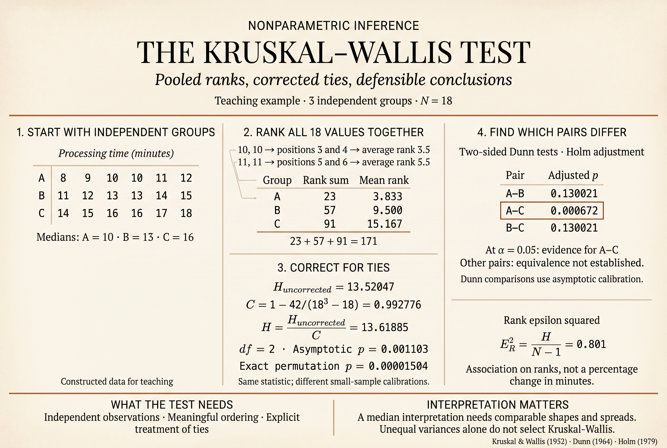
Consider processing time, in minutes, under three protocols A, B, and C. Each group represents six different units. The data are constructed for teaching; they are not research observations or evidence about an actual service. Rows are arranged for readability only and do not imply matching across groups.
| Row | A: min | A: rank | B: min | B: rank | C: min | C: rank |
|---|---|---|---|---|---|---|
| 1 | 8 | 1 | 11 | 5.5 | 14 | 11.5 |
| 2 | 9 | 2 | 12 | 7.5 | 15 | 13.5 |
| 3 | 10 | 3.5 | 13 | 9.5 | 16 | 15.5 |
| 4 | 10 | 3.5 | 13 | 9.5 | 16 | 15.5 |
| 5 | 11 | 5.5 | 14 | 11.5 | 17 | 17 |
| 6 | 12 | 7.5 | 15 | 13.5 | 18 | 18 |
The value 10 occupies positions 3 and 4, so both observations receive rank 3.5. The value 11 occupies positions 5 and 6, receiving rank 5.5 even though one observation belongs to A and the other to B. This second case shows why groups must be pooled before assigning ranks.
| Group | n | Median | Q1 | Q3 | IQR | Rank sum | Mean rank |
|---|---|---|---|---|---|---|---|
| A | 6 | 10 | 9.25 | 10.75 | 1.50 | 23 | 3.833333 |
| B | 6 | 13 | 12.25 | 13.75 | 1.50 | 57 | 9.500000 |
| C | 6 | 16 | 15.25 | 16.75 | 1.50 | 91 | 15.166667 |
IQR = Q3 − Q1. Interpolated quartiles are meaningful for these quantitative times; a purely ordinal scale would call for categories and an appropriate quantile convention. The samples intentionally share the same shifted empirical pattern, which establishes nothing about population distributional shapes.
06. Complete calculation
Here k = 3, N = 18, and nA = nB = nC = 6. The rank sums are 23, 57, and 91. As a check, they sum to 171 = 18 × 19 / 2.
= 13.52046784.
Seven values occur twice each: 10, 11, 12, 13, 14, 15, and 16. Values 8, 9, 17, and 18 occur only once.
C = 1 − 42183 − 18 = 0.9927760578.
With two degrees of freedom, the chi-squared survival function simplifies to exp(−H/2). Therefore:
= 0.00110332734 ≈ 0.00110.
At a prespecified α = .05, the global null is rejected using asymptotic calibration. The evidence concerns the group collection: it does not yet identify different pairs. Moreover, six units per group make a permutation check of the approximation worthwhile, without conflating the resulting p-values.
07. Dunn comparisons and Holm adjustment
Dunn comparisons locate differences while retaining the pooled sample ranks and incorporating a tie correction (Dunn, 1964). We declare a family of three two-sided comparisons: A–B, A–C, and B–C.
zij = R̄i − R̄j√[Vr(1/ni + 1/nj)].
The common standard error is √[28.29411765(1/6 + 1/6)] = 3.07105398. For A–C, the mean-rank difference is −11.33333333, giving z = −3.69037256. Unadjusted two-sided p-values are computed as 2Φ(−|z|).
| Pair | z | Unadjusted p | Holm p | Decision, α = .05 |
|---|---|---|---|---|
| A–B | −1.84518628 | 0.06501045 | 0.13002089 | Do not reject |
| A–C | −3.69037256 | 0.00022393 | 0.00067178 | Reject |
| B–C | −1.84518628 | 0.06501045 | 0.13002089 | Do not reject |
Holm sorts p-values from smallest to largest, applies multipliers 3, 2, and 1, then takes cumulative maxima to preserve ordering. Here this gives 3 × 0.00022392585 = 0.00067177756 and, for the other two pairs, 2 × 0.06501044574 = 0.13002089148. The last adjusted value stays at that cumulative maximum instead of falling to 0.06501045.
Holm controls the family-wise error rate under arbitrary dependence among tests, provided the individual p-values are validly calibrated; Dunn uses a normal approximation here (Holm, 1979; R Core Team, n.d.-a). The adjustment therefore does not remove small-sample limitations.
This exploratory strategy reports Dunn after global rejection. Prespecified contrasts can be organized under a different inferential plan; declare the comparison family and multiplicity control before selecting results. Pairwise Wilcoxon tests with their own reranking can form a different strategy, but should not be presented as Dunn comparisons.
08. Effect size
A difference can be statistically detectable yet practically small. Here the declared index is rank epsilon squared, using the convention E²R = H/(N − 1). It is a rank-based association measure, rather than a percentage change in minutes.
Its descriptive meaning can be checked without an automatic “small” or “large” label. With r̄ = (N + 1)/2 = 9.5:
SStotal = Σi,j(rij − r̄)2 = 481,
SSbetweenSStotal = 0.80110880 = ER2.
The identity holds when H includes the tie correction. In this sample, the index equals the fraction of rank variability associated with the group partition. It does not mean that the protocol causally explains 80.1% of original processing times or reduces times by 80.1%. Generalizing the magnitude requires uncertainty assessment and a suitable design.
Terminology varies across texts and software. A related index, η²H = (H − k + 1)/(N − k), equals 0.77458997 here. It is not interchangeable with E²R; it can even yield negative estimates when H is small. Functions in effectsize distinguish these conventions, and formulas should accompany any report (Ben-Shachar et al., 2020; easystats, n.d.).
On the original scale, the medians are 10, 13, and 16 minutes; the descriptive C − A difference is 6 minutes. This difference between sample medians is not a Hodges–Lehmann shift estimate, and Dunn’s p-value does not provide a confidence interval for it.
09. Reproducible R code
The following code uses only base R and its included stats package. It constructs the data, prints descriptive statistics, computes H, checks agreement with kruskal.test(), performs two-sided Dunn comparisons with Holm adjustment, and verifies the effect-size identity.
dat <- data.frame(
  group = factor(rep(c("A", "B", "C"), each = 6)),
  time = c(8, 9, 10, 10, 11, 12,
           11, 12, 13, 13, 14, 15,
           14, 15, 16, 16, 17, 18)
)
stopifnot(is.numeric(dat$time), all(is.finite(dat$time)),
          !anyNA(dat$group), nlevels(dat$group) >= 2)
g <- droplevels(dat$group)
x <- dat$time
N <- length(x)
k <- nlevels(g)
n <- table(g)
stopifnot(all(n > 0), N > k)
r <- rank(x, ties.method = "average")
Rsum <- tapply(r, g, sum)
Rmean <- tapply(r, g, mean)
desc <- t(vapply(split(x, g), function(v) {
  q <- quantile(v, c(0.25, 0.75), type = 7, names = FALSE)
  c(n = length(v), median = median(v), Q1 = q[1],
    Q3 = q[2], IQR = q[2] - q[1])
}, numeric(5)))
print(desc)
print(data.frame(dat, rank = r))


tied_n <- as.numeric(table(x))
Tsum <- sum(tied_n^3 - tied_n)
Ctie <- 1 - Tsum / (N^3 - N)
if (Ctie <= 0) stop("All observations are tied")
H_uncorrected <- 12 / (N * (N + 1)) * sum(Rsum^2 / as.numeric(n)) - 3 * (N + 1)
H <- H_uncorrected / Ctie
p_asymptotic <- pchisq(H, df = k - 1, lower.tail = FALSE)
kw <- kruskal.test(time ~ group, data = dat)
stopifnot(isTRUE(all.equal(H, unname(kw$statistic), tolerance = 1e-12)),
          isTRUE(all.equal(p_asymptotic, kw$p.value, tolerance = 1e-12)))
print(kw)
print(c(Tsum = Tsum, Ctie = Ctie, H_uncorrected = H_uncorrected,
        H = H, p_asymptotic = p_asymptotic))


Vrank <- N * (N + 1) / 12 - Tsum / (12 * (N - 1))
pairs <- combn(levels(g), 2)
post <- do.call(rbind, lapply(seq_len(ncol(pairs)), function(j) {
  a <- pairs[1, j]
  b <- pairs[2, j]
  se <- sqrt(Vrank * (1 / n[a] + 1 / n[b]))
  z <- unname((Rmean[a] - Rmean[b]) / se)
  data.frame(pair = paste(a, b, sep = "-"), z = z,
             p_raw = 2 * pnorm(abs(z), lower.tail = FALSE))
}))
rownames(post) <- NULL
post$p_holm <- p.adjust(post$p_raw, method = "holm")
print(post, digits = 9)


epsilon_rank <- H / (N - 1)
eta_H <- (H - k + 1) / (N - k)
SS_between <- sum(as.numeric(n) * (Rmean - mean(r))^2)
SS_total <- sum((r - mean(r))^2)
stopifnot(isTRUE(all.equal(epsilon_rank,
                         unname(SS_between / SS_total), tolerance = 1e-12)))
print(c(epsilon_rank = epsilon_rank, eta_H = eta_H,
        SS_between = SS_between, SS_total = SS_total))
Reference results: H = 13.61884962; df = 2; p = 0.00110332734; E²R = 0.80110880. Holm-adjusted p-values, in A–B, A–C, B–C order, are 0.13002089, 0.00067178, and 0.13002089. The complete calculations were executed in R 4.6.0 and independently cross-checked with Python/SciPy; the last printed decimal places may vary.
The block rejects missing and nonfinite values so that the analyzed sample is explicit. With other data, decide and document missing-data treatment before analysis. For ordinal responses, use numerical codes that respect the ordering, rather than arbitrary conversions of labels.
10. Permutation calibration and uncertainty
Permutation calibration
Under the null of identical distributions and independent observations, group labels are exchangeable while their sizes are held fixed. Ranks can be permuted among group positions, keeping C fixed and recalculating H. If assignment is restricted or the design includes blocks or clusters, permutations must respect those restrictions; shuffling all labels is insufficient.
The next block draws B = 99,999 random permutations with replacement across draws; each draw redistributes the N observations without replacement. If b simulated statistics are at least as extreme as the observed statistic, use (b + 1)/(B + 1), including the observed configuration. This avoids reporting zero merely because few simulations were run (Phipson & Smyth, 2010).
Run this block after the preceding code. The 10−10 tolerance prevents floating-point rounding from excluding numerical ties. The second part exhaustively enumerates partitions of this balanced example; its restriction to three groups of six observations is checked explicitly in the code.
set.seed(20261110)
B <- 99999L
H_perm <- replicate(B, {
  rp <- sample(r, N, replace = FALSE)
  sp <- tapply(rp, g, sum)
  (12 / (N * (N + 1)) * sum(sp^2 / as.numeric(n)) - 3 * (N + 1)) / Ctie
})
b <- sum(H_perm >= H - 1e-10)
p_MC <- (b + 1) / (B + 1)
MCSE <- sqrt(p_MC * (1 - p_MC) / B)
print(c(B = B, b = b, p_MC = p_MC, MCSE = MCSE))

stopifnot(N == 18L, k == 3L, all(n == 6L))
r2 <- as.integer(2 * r)
target <- sum((2 * Rsum)^2)
A_choices <- combn(2:18, 5)
B_template <- combn(2:12, 5)
extreme <- 0
total <- 0
for (j in seq_len(ncol(A_choices))) {
  ia <- c(1L, A_choices[, j])
  rest <- r2[-ia]
  sa <- sum(r2[ia])
  sb <- rest[1] + colSums(matrix(rest[B_template], nrow = 5))
  sc <- sum(r2) - sa - sb
  extreme <- extreme + sum(sa^2 + sb^2 + sc^2 >= target)
  total <- total + length(sb)
}
p_exact <- extreme / total
stopifnot(total == 2858856, extreme == 43)
print(c(partitions = total, extreme_partitions = extreme,
        labeled_allocations = 6 * total, p_exact = p_exact))
The first part of the output gives B, b, the Monte Carlo p-value, and its approximate standard error. That error describes simulation variability only, rather than the study’s sampling uncertainty. Monte Carlo provides an alternative calibration of the same H; it need not equal the asymptotic value 0.00110332734, and the smaller of the two should not be selected. The preceding Dunn comparisons remain asymptotic.
An exhaustive check for this example
Equal group sizes make H invariant to exchanging group names. The code fixes the first unit in A and the first remaining unit in B, enumerating each unlabeled partition once. There are 2,858,856 partitions, equivalent to 17,153,136 labeled allocations, six per partition. Tied observations remain distinct units with equal values, preserving allocation probabilities.
Exactly 43 partitions have H at least as large as observed: pexact = 43/2,858,856 = 258/17,153,136 = 0.00001504098. The comparison doubles the ranks and uses integer arithmetic to count extremes without floating-point ambiguity. Because enumeration includes every configuration and the observed one, no further unit is added to the numerator.
With the stated seeds, R 4.6.0 produced b = 3 and pMC = 0.00004000, with SEMC ≈ 0.00002000. Only three exceedances mean poor relative precision: this short simulation cannot estimate such a small value closely. Exhaustive enumeration does determine its exact conditional value. All three calibrations reject at .05, but their magnitudes differ substantially. Enumeration is preferred in this example because it is feasible and avoids approximation and Monte Carlo error, rather than because it yields the smallest p-value.
Effect-size uncertainty
The next supplement computes an exploratory 95% percentile interval for E²R. It resamples within each group, holds group sizes fixed, and recomputes ranks in every replicate. This addresses a different question from permutation: assessing variability around the observed empirical distributions without imposing identical groups.
set.seed(20261111)
B_boot <- 3999L
xb <- split(x, g)
epsilon_boot <- replicate(B_boot, {
  samples <- lapply(xb, function(v) sample(v, length(v), replace = TRUE))
  y <- unlist(samples, use.names = FALSE)
  if (length(unique(y)) < 2L) return(NA_real_)
  as.numeric(kruskal.test(samples)$statistic) / (N - 1)
})
CI_percentile <- quantile(epsilon_boot, c(0.025, 0.975),
                          na.rm = TRUE, type = 7)
print(CI_percentile)
print(c(valid_bootstrap = sum(is.finite(epsilon_boot))))
sessionInfo()
With only six observations per group, bootstrap sampling reproduces highly discrete empirical distributions. Coverage can be poor and index bias can remain; the interval is not a guarantee of population precision. In R 4.6.0, all 3,999 replicates were valid and yielded the exploratory interval [0.6908765, 0.9104320]. Exclusion of zero must not be used as a test for the presence or absence of association: for bounded indices, bootstrap intervals can exclude zero even under the null (easystats, n.d.). The code prints the number of valid replicates, and sessionInfo() records the environment. Confirmatory conclusions about magnitudes or equivalence require planning the estimand, interval procedure, and sample size specifically.
11. Reporting the result
A report should connect design, descriptive statistics, calibration, multiplicity, and limitations. For this constructed example, one possible report is:
If only Monte Carlo calibration is available, replace the exact value with its corresponding output and report the number of draws, seed, and a measure of simulation precision. A value computed from a random sample of permutations should not be described as “exact” without exhaustive enumeration.
| Avoid | Defensible statement |
|---|---|
| “The probability that H₀ is true is .00110.” | “Under H₀ and the test conditions, the probability of an H at least this extreme is approximately .00110.” |
| “All three groups differ.” | “The global null is rejected; Dunn with Holm provides evidence for A–C.” |
| “A and B are equal because p > .05.” | “There was insufficient evidence to reject that comparison; equivalence was not established.” |
| “The effect explains 80.1% of processing time.” | “Rank epsilon squared is .801; its scale and denominator are stated explicitly.” |
| “The median in C is causally six minutes higher.” | “The descriptive difference between sample medians in C and A is six minutes; causality depends on design.” |
Medians and IQRs are often informative, but do not prohibit adding means, standard deviations, or other summaries when useful. Descriptive choices should follow the measurement scale, distribution, and question, rather than an automatic obligation imposed by a test name.
12. Methodological scope
Ranks are an abstraction from data: they preserve order relations while discarding some distance information. That abstraction is appropriate only in relation to the research object and question. For waiting times, identifying who tends to wait longer may matter; for public budgets, an absolute monetary difference can be decisive and insufficiently represented by ordering.
Likewise, a statistical category does not itself explain the mechanism producing its differences. Rank comparisons among establishments, sectors, or territories cannot replace investigation of resources, work organization, participant selection, and historical conditions. A test contributes evidence about an observed structure under explicit assumptions; explanation requires theory, contextual knowledge, and a design capable of supporting it.
A defensible workflow is concrete: define the unit and question; examine distributions and measurement; choose a test coherent with the design; verify calculations; quantify uncertainty; and match conclusions to the available information. Used this way, Kruskal–Wallis becomes a precise tool rather than an automatic response to any ANOVA assumption violation.
13. References
Ben-Shachar, M. S., Lüdecke, D., & Makowski, D. (2020). effectsize: Estimation of effect size indices and standardized parameters. Journal of Open Source Software, 5(56), Article 2815. https://doi.org/10.21105/joss.02815
Dunn, O. J. (1964). Multiple comparisons using rank sums. Technometrics, 6(3), 241–252. https://doi.org/10.1080/00401706.1964.10490181
easystats. (n.d.). Effect size for rank based ANOVA [effectsize package documentation]. Retrieved November 10, 2026, from https://easystats.github.io/effectsize/reference/rank_epsilon_squared.html
Holm, S. (1979). A simple sequentially rejective multiple test procedure. Scandinavian Journal of Statistics, 6(2), 65–70. https://www.jstor.org/stable/4615733
Kruskal, W. H., & Wallis, W. A. (1952). Use of ranks in one-criterion variance analysis. Journal of the American Statistical Association, 47(260), 583–621. https://doi.org/10.1080/01621459.1952.10483441
National Institute of Standards and Technology. (n.d.). Kruskal Wallis. Dataplot reference manual. Retrieved November 10, 2026, from https://www.itl.nist.gov/div898/software/dataplot/refman1/auxillar/kruskwal.htm
Phipson, B., & Smyth, G. K. (2010). Permutation p-values should never be zero: Calculating exact p-values when permutations are randomly drawn. Statistical Applications in Genetics and Molecular Biology, 9(1), Article 39. https://doi.org/10.2202/1544-6115.1585
R Core Team. (n.d.-a). Adjust p-values for multiple comparisons [R documentation]. Retrieved November 10, 2026, from https://stat.ethz.ch/R-manual/R-devel/library/stats/html/p.adjust.html
R Core Team. (n.d.-b). Friedman rank sum test [R documentation]. Retrieved November 10, 2026, from https://stat.ethz.ch/R-manual/R-devel/library/stats/html/friedman.test.html
R Core Team. (n.d.-c). Kruskal-Wallis rank sum test [R documentation]. Retrieved November 10, 2026, from https://stat.ethz.ch/R-manual/R-devel/library/stats/html/kruskal.test.html
R Core Team. (n.d.-d). Test for equal means in a one-way layout [R documentation]. Retrieved November 10, 2026, from https://stat.ethz.ch/R-manual/R-devel/library/stats/html/oneway.test.html
Welch, B. L. (1951). On the comparison of several mean values: An alternative approach. Biometrika, 38(3–4), 330–336. https://doi.org/10.2307/2332579
Documentation pages are changing resources; accessed November 10, 2026. Letters a–d follow alphabetical title order. For computational definitions of E²R and η²H, see also the official effectsize documentation. Formulas are stated explicitly to avoid naming ambiguity.
Leave a Comment/Deja un Comentario