
Marxist philosophy of science · Mathematics notebook
Algebraic Structures
Structure, invariance, and transformation from the standpoint of dialectical materialism
Originally published:
Revised and expanded edition:
Abstract
A mathematical structure is identified through the relations it organizes and the transformations that preserve them. This essay examines operations, groups, rings, and fields; connects algebras of sets with measure and probability; and develops a dialectical-materialist interpretation of essence as the articulation of structural layers. The discussion of quantity, quantum, degree, and measure culminates in two applications: qualitative transformation in a dynamical system and the construction of σ-additive functions associated with additive genetic models. In each case, the objects, assumptions, and scope of inference are specified.
Concepts: abstract algebra · isomorphism · essence · invariants · σ-algebra · measure · quantitative genetics · dialectical materialism
I · The problem
Knowing an object means investigating its relations
A collection of elements does not exhaust our knowledge of a system. What matters includes the relations among its components, the operations that can be performed on them, and the conditions under which the whole preserves or transforms its organization. The difference between an inventory and a structure raises a question shared by abstract algebra and materialist philosophy: what determines that something is the system it is?
Algebra answers by specifying operations and axioms. Concrete scientific investigation must also explain how its objects acquire those relations, which processes reproduce them, and under what conditions they change. Dialectical materialism provides an orientation here: to study objects through their connections, motion, and historical determinations. Mathematical formalization makes aspects of those connections precise and allows the consequences of explicit assumptions to be proved.
From this perspective, historical materialism provides categories for investigating the organization and transformation of societies, while dialectical materialism guides reflection on the more general relations among structure, process, and knowledge. An algebraic identity can contribute to a social model; its explanatory relevance depends on historical mediations and investigation of the object. The social content of a relation of production requires determinations that cannot be obtained from its formal expression alone.
In the introduction of 1857, Marx develops the problem of intellectually reconstructing a concrete whole comprising multiple determinations. We take up that orientation to ask what each structure abstracts and what must be restored to understand a concrete system (Marx, 1973, Introduction, § 3). The exposition proceeds from elementary operations to questions of measure and modeling, maintaining three questions: what is defined, what is proved, and what interpretation is proposed.
II · Language and operations
From operands to composition laws
2.1. Function, operation, operator, and symbol
A function f: A → B assigns a unique element of its codomain B to each element of its domain A. The arrow indicates this assignment between sets. It should be distinguished from logical implication, usually written ⇒. The domain, codomain, and assignment rule are part of the specification of a function.
An operation combines inputs to produce an output. Its inputs are called operands; the sign used to represent it is its symbol. In a + b, the operands are a and b, and + represents addition. The same notation may denote different operations on numbers, matrices, or functions; its meaning comes from the specified structure.
The term operator depends on context. In functional analysis it often denotes a map between function spaces or vector spaces, frequently a linear one. A linear operator on V is a linear endomorphism T: V → V. The word map is a general term for function, even when its domain and codomain differ. Identifying an operator with its symbol is insufficient when studying its mathematical properties.
2.2. Internal operations
An internal binary operation on a set A is a function of two arguments whose values belong to A:
The symbol A × A represents the Cartesian product: the set of ordered pairs of elements of A. Closure is built into the codomain. Integer addition is internal to ℤ; division does not define a total internal operation on ℤ, because some quotients are not integers and division by zero is excluded.
A function A × B → C is generally a two-argument operation with possibly different input and output types. An internal operation on a single set is obtained only when these three roles are appropriately identified. Distance between points in the plane, for example, has type d: ℝ2 × ℝ2 → [0,∞): it produces a number from two points. This function is not a group operation on the points of the plane.
2.3. Left and right external operations
An external operation relates elements of sets playing different roles. For a scalar set K and a set V, the usual forms are:
Input and output types must remain consistent. Furthermore, a map of this type becomes a group action or scalar multiplication for a module or vector space when it satisfies the corresponding axioms. The function type alone is insufficient. “External” describes the structural roles of the operands; it does not require their underlying sets to be disjoint.
2.4. What an algebraic structure contains
In the elementary case, an algebraic structure consists of a nonempty set with specified operations, together with axioms determining the class under consideration. We may write (A,∗) or (A,+,·,0,1). A tuple records the data; the axioms express their relations. There are also structures with several underlying sets, such as a vector space and its scalar field.
This observation raises a philosophical question: structural identity depends on the relations selected. The same set of integers can be studied as a set, an additive group, a ring, or an ordered set. Each choice preserves information and abstracts from other determinations. Scientific knowledge requires a justification of why those relations are relevant to the problem being investigated.
III · Fundamental structures
Groups, rings, fields, and vector spaces
3.1. Groups and abelian groups
A group (G,∗) has an associative internal binary operation, an identity element, and an inverse for every element. For any a,b,c ∈ G:
Identity and inverse are defined with respect to an operation. In (ℤ,+), the identity is 0 and the inverse of a is −a. In (ℝ ∖ {0},·), they are 1 and 1/a. A group is abelian if it also satisfies a ∗ b = b ∗ a.
The bijections of a set onto itself form a group under composition. Composition allows the inverse to be interpreted as an operation that reverses another transformation. In noncommutative groups, composition order affects the result; certain rotations of three-dimensional space provide an example. This dependence on order can model aspects of concrete processes when the operations and their conditions have been identified.
3.2. Rings and semirings
We adopt the convention that a ring R is associative and has a multiplicative identity. Its addition forms an abelian group; its multiplication is associative; and the operations are related by the distributive laws:
In particular, a + 0 = 0 + a = a, whereas a + (−a) = 0. A ring is commutative when its multiplication is commutative. Rings without identity are also studied; they will be explicitly identified when they appear. Such conventions must remain consistent throughout an exposition (Milne, 2022, “Rings” section).
The integers form a commutative ring: (ℤ,+,·). Square matrices of size n ≥ 2 with real entries form a generally noncommutative ring. Distributive compatibility allows two kinds of operation to be combined on the same underlying set. A ring has an underlying additive group; multiplication adds structure.
An algebraic semiring, under the usual convention with identity, replaces the additive group with a commutative monoid: it retains associative addition, zero, and commutativity, but does not require additive inverses. Multiplication is associative with identity, distributes over addition, and has zero as an absorbing element. (ℕ0,+,·) is an example. We will later encounter a semiring of sets, a term used in measure theory with a specific definition.
3.3. Fields, division rings, and algebras
A field F is a commutative ring with 1 ≠ 0 in which every nonzero element has a multiplicative inverse. Equivalently, (F,+) and (F ∖ {0},·) must be abelian groups compatible through distributivity. The rational, real, and complex numbers are examples.
In a division ring, nonzero elements are invertible and multiplication may be noncommutative. The quaternions provide an example. An algebra over a field additionally incorporates a vector-space structure and a bilinear multiplication. A division algebra is defined in that context; the scalar field and associativity conventions should therefore be specified, rather than using all these names interchangeably.
| Structure | Operations and requirements | Example |
|---|---|---|
| Abelian group | One internal operation with associativity, identity, inverses, and commutativity. | (ℤ,+) |
| Ring | An additive abelian group and an associative, distributive multiplication; here, with identity. | ℤ; matrices M2(ℝ) |
| Field | A commutative ring, 1 ≠ 0, and multiplicative inverses for nonzero elements. | ℚ, ℝ, ℂ |
| Vector space | An additive abelian group and external multiplication by a field, satisfying the compatibility axioms. | ℝ2 over ℝ |
3.4. Vector spaces, modules, and Hilbert spaces
A vector space V over F has internal addition and external scalar multiplication. For scalars λ,η and vectors u,v:
Multiplication of two vectors is not part of those axioms. A field is a vector space over itself and, more generally, over any of its subfields; this expresses a relation between specified structures. A module generalizes scalar multiplication by replacing the field with a ring, with distinctions between left and right modules when multiplication is noncommutative.
An inner product allows the norm ‖v‖ = √⟨v,v⟩ and distance d(u,v) = ‖u−v‖ to be defined. A Hilbert space is an inner-product space complete in that norm: every Cauchy sequence converges in the space. It may be finite- or infinite-dimensional; separability is an additional property. In finite dimensions, a real Euclidean space with its inner product is a special case.
IV · Preservation and history
Isomorphisms and the formation of the concept of structure
4.1. What a homomorphism preserves
A group homomorphism f: G → H preserves the operation:
If it is bijective, it is a group isomorphism. Its inverse also preserves the operation. A ring isomorphism must preserve both operations and, under our convention, the identity. An automorphism is an isomorphism of a structure onto itself; an endomorphism is a homomorphism from a structure to itself.
“Classification up to isomorphism” means identifying structures that are equivalent with respect to the type of structure under consideration. For example, a group isomorphism preserves the order of each element and commutativity. It need not preserve an additional distance that is not part of the algebraic data. For more general relational structures, preservation and reflection of relations must also be specified.
Three related concepts should be distinguished: the inverse of an element with respect to an operation, the inverse of a function, and an isomorphism as a structure-preserving correspondence. Inverse functions satisfy f-1 ∘ f = id; isomorphisms add preservation requirements. This precision allows the philosophical relation between reversibility and identity to be developed without making the entire notion of structure depend on a single kind of inverse.
4.2. Example: transforming addition into multiplication
Consider f(x) = ex from the real numbers with addition to the positive real numbers with multiplication:
The exponential is bijective on these domains, with the logarithm as its inverse. The two groups are therefore isomorphic. Addition on one side corresponds to multiplication on the other: symbols and elements differ, but the composition law is transported exactly. This equivalence concerns the group; it does not assert that the exponential preserves Euclidean distance.
4.3. A history involving several mediations
The modern notion of structure emerged through interactions among algebraic, geometric, physical, and philosophical problems. Timmermans’s historical study reconstructs connections among crystallography, transformation groups, and philosophy; it also shows that the historical meaning of “isomorphism” was not uniform. Correspondences called holohedral and merihedral cannot simply be translated into current terminology (Timmermans, 2012).
This development includes Leibniz’s ideas of similarity, the study of crystal symmetries, and the subsequent elaboration of groups and composition relations. Weyl connected structure with isomorphism in a text of 1927; in the twentieth century, Bourbaki systematized a perspective in which the type of structure determines its admissible correspondences. This history requires distinguishing the first appearance of a word, the study of particular cases, and the formulation of a general definition.
Crystallography is particularly significant for a materialist interpretation: spatial arrangements and symmetry operations provided problems that stimulated structural abstraction. When applied to other domains, abstraction preserves selected relations and makes new consequences available for investigation. Its emergence and application in turn require specific historical inquiry.
In the Soviet philosophical tradition, the entries “Structure” and “Isomorphism” connect the stability of relations with modeling and knowledge of the object. The 1984 reworking emphasizes the multiplicity of structures within a single system and the transformation of its relations (Rosental & Iudin, 1965; Frolov, 1984). This perspective makes it possible to move from abstract structure to the question of how its determinations are materially articulated.
V · Essence and determinations
Essence as the articulation of structural layers
5.1. A unity with several determinations
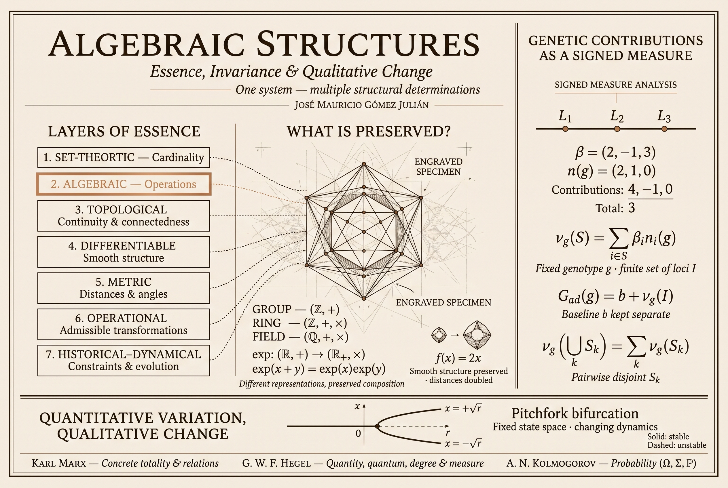
The analysis of essence can be organized through mathematical layers specifying constitutive relations and invariants. This formulation, developed in the manuscript Geometry, History, and Lawfulness, allows the same object to be investigated through distinct, articulated determinations (Gómez Julián, 2026, §§ 1.2–1.8). The algebraic layer is central here: it identifies operations and compatibilities that cannot be reduced to the number of elements or to a geometric outline.
A layer expresses an aspect of the object’s organization and the type of transformation under which it is preserved. Articulating layers requires dependencies to be specified: a Riemannian metric is defined on a smooth manifold; an algebraic structure can be studied with or without a compatible topology; the history of a process may require additional information about causality and inherited constraints. The same system is thus investigated through different levels of determination.
| Layer | What is specified and preserved | Relevant transformation |
|---|---|---|
| Set-theoretic | Correspondence between elements and cardinality. | Bijection. |
| Algebraic | Operations and composition relations. | Isomorphism of the relevant algebraic type. |
| Topological | Open sets, continuity, connectedness, and compactness. | Homeomorphism. |
| Differentiable | Smooth structure and compatible differential calculus. | Diffeomorphism. |
| Metric | Distances; in Riemannian geometry, the metric tensor, lengths, and angles. | Isometry. |
| Operational | Composition of admissible transformations and symmetries. | Automorphisms; groups and actions when their axioms hold. |
| Historical and dynamical | Causal relations, inherited constraints, and the law of evolution. | Maps preserving historical data and intertwining the specified dynamics. |
In this interpretation, preserved properties help delimit what counts as identity at a given level. The choice of level arises from the object and the problem. Comparing concrete phenomena requires establishing which essential aspects the model captures and which remain outside its representation. An isolated invariant may be informative without completely classifying a structure: equal cardinality does not determine equal topology or an identical operation.
5.2. Preserving more structure restricts transformations
On a fixed smooth manifold M, equipped with a Riemannian metric g, the following inclusions hold:
A Riemannian isometry is a diffeomorphism preserving the metric tensor; every diffeomorphism is a homeomorphism; and every homeomorphism is a bijection. If one begins with a bijection preserving Riemannian distance, its smoothness is a regularity result, not a consequence obtained simply by writing derivatives of a function not yet known to be differentiable.
The inclusions can be strict, but this must be checked for the object under consideration. Adding structure does not automatically generate a new space through an arrow: a bijection does not produce a topology, nor does a homeomorphism by itself add a differentiable structure. The definitions of manifolds and smooth maps rely on explicit data and compatibilities (Meinrenken, 2001, § 1).
Three transformations of the real line
Dilation: f(x)=2x is a diffeomorphism of ℝ with inverse x/2, but it doubles Euclidean distances. It also preserves addition, so it is an automorphism of the additive group.
Cubic map: h(x)=x3 is a homeomorphism of ℝ. Its inverse, the cube root, is not differentiable at zero; hence h is not a diffeomorphism. It does not preserve addition either.
Swapping points: the bijection that swaps 0 and 1 and fixes every other real number is discontinuous. It preserves cardinality, but not the usual topology.
These examples show that preservation depends on the relations considered. A metric variation can leave topological identity intact; modifying the composition law can change algebraic identity on the same underlying set. Qualitative transformation must be located in the determination that actually changes.
5.3. Operational essence and history
The automorphisms of a structure form a group under composition. This group organizes reversible transformations preserving the specified data and provides a formalization of operational essence. Adding a smooth structure and compatibility with multiplication and inversion may produce a Lie group. The Lie-group condition must be established; an abstract automorphism group does not possess it automatically (Meinrenken, 2002, § 10).
History introduces another question: how were the relations that now admit those symmetries formed? In a dynamical model, a transformation h is compatible with the evolution Φt when h ∘ Φt = Φt ∘ h. When two different dynamics are compared, the corresponding equation is a conjugacy or an intertwining relation between their evolutions. Preserving the instantaneous metric is insufficient to preserve an additional law of motion.
Processes involving memory, accessibility constraints, or information loss may require an enlarged state space or the use of semigroups, categories, or groupoids. That choice is justified by examining composition, identity, and invertibility. A layered formulation allows preservation and transformation to be investigated without assuming that every historical evolution is a symmetry group.
VI · Algebra of sets
The power set and its operations
6.1. From elements to subsets
The power set of X is the collection of all its subsets, written ℘(X) or 2X. For a finite set with n elements, it contains 2n subsets: each element can independently be included or excluded.
The empty set is a subset of every set. This does not imply that it is an element of every set: ∅ ⊆ X and ∅ ∈ X are different statements. By contrast, ∅ ∈ ℘(X) always holds. This distinction between membership and inclusion is indispensable when studying systems whose elements are themselves sets.
6.2. Symmetric difference as addition
The symmetric difference consists of the elements belonging to one of two sets but not to both:
On ℘(X), symmetric difference is associative and commutative, has identity ∅, and makes every set its own inverse: A △ A = ∅. Thus (℘(X),△) is an abelian group. Adding intersection as multiplication gives a commutative ring with identity X.
Union is recovered through A ∪ B = (A △ B) △ (A ∩ B), and difference through A ∖ B = A △ (A ∩ B). These identities explain the connection between set operations and ring structure. Union does not play the role of addition with inverses in this ring.
6.3. Rings, semirings, and algebras of sets
A ring of sets is a nonempty family closed under finite union and difference. Equivalently, it is closed under symmetric difference and intersection. It may fail to contain the ambient set X: the family of all finite subsets of an infinite set is an example. As a Boolean ring, it may have no identity of its own.
An algebra of sets on X contains X and is closed under complements relative to X and finite unions. Closure under intersection follows from De Morgan’s laws. Its identity is the greatest element of the family under inclusion, since it contains every member.
A semiring of sets contains ∅, is closed under intersections, and allows the difference of two members to be written as a finite disjoint union of members of the family. Bounded half-open intervals [a,b), together with the empty set, provide an example on ℝ. This decomposition permits measures to be constructed from elementary pieces, as studied by Kolmogórov and Fomin (1978, chap. I, § 5).
VII · Order relations
Partial order, extremal elements, and generation
7.1. Ordering does not always make everything comparable
A partial order ≤ is a reflexive, antisymmetric, and transitive relation. Reflexivity means a ≤ a; antisymmetry means that a ≤ b and b ≤ a imply a=b; transitivity means that a ≤ b ≤ c implies a ≤ c. Set inclusion is a partial order.
In a total order, any two elements are comparable. A well-order additionally requires every nonempty subset to have a least element. The real numbers with their usual order are totally ordered but not well-ordered: the interval (0,1) has no least element. For finite sets, every total order is a well-order.
| Concept | Condition |
|---|---|
| Greatest element m | a ≤ m for every a ∈ P. |
| Maximal element m | If m ≤ a, then a = m. |
| Least element m | m ≤ a for every a ∈ P. |
| Minimal element m | If a ≤ m, then a = m. |
Every greatest element is maximal; the converse can fail. The family {{a},{b}}, ordered by inclusion with a≠b, has two maximal elements and no greatest element. The family {∅,{a},{b},{a,b}} does have a greatest element: {a,b}. Greatest and least elements, when they exist, are unique. In a total order, a maximal element is greatest, but there need not be any.
7.2. The smallest system containing specified data
This precision is useful when constructing a generated structure. Fix an ambient set X and a family 𝒞 ⊆ ℘(X). The σ-algebra generated by 𝒞 is the intersection of all σ-algebras on X containing it:
The family being intersected is nonempty, because ℘(X) is a σ-algebra containing 𝒞. Its intersection preserves the axioms. The result is the least σ-algebra under inclusion containing the generators, not merely a minimal element among the candidates (Viaclovsky, 2003, Proposition 0.3).
Older expositions may distinguish a family with no points outside the union of its generators from the smallest closed family containing them. The first issue fixes the ambient set; the second fixes the collection of admissible subsets. This distinction avoids importing concepts of “minimal algebra” from other fields as though they were equivalent to a generated σ-algebra.
VIII · Events and topology
σ-algebras, Borel sets, and probability
8.1. The three axioms
A σ-algebra Σ on X is a collection of subsets with the following properties:
These axioms imply membership of the empty set and closure under countable intersections and differences. “Countable” here refers to the sequence of sets being operated on. It does not require each set to have countably many points, nor does it require the σ-algebra itself to be a countable collection.
De Morgan’s identities provide the connection among complements, unions, and intersections:
A σ-ring is a ring of sets closed under countable unions; a δ-ring is closed under countable intersections. When the ring contains the ambient set and therefore relative complements, these two closure properties are connected by those identities. Duality transforms one operation into another through complementation: it does not identify union with intersection.
8.2. What makes a σ-algebra a Borel σ-algebra
If (X,τ) is a topological space, its Borel σ-algebra is generated by its open sets:
It can also be generated by the closed sets. The definition depends on the chosen topology and applies to general spaces, not only to the real line. On ℝ with its usual topology, it contains intervals and many other sets of points. A Borel set can be uncountable: [0,1] is an example.
Some historical texts use “B-algebra” or “Borel algebra” in a broader sense close to an abstract σ-algebra. This edition uses the current distinction: Σ denotes a σ-algebra; ℬ(X) denotes the σ-algebra generated by a topology. This preserves the historical reading of Kolmogórov and Fomin without attributing an unspecified topology to every σ-algebra.
8.3. Sample space and probability
A probability space is a triple (Ω,Σ,ℙ): Ω contains the possible outcomes, Σ contains the measurable events, and ℙ assigns them probabilities σ-additively, with ℙ(Ω)=1. The sample space may describe physical outcomes, sequences, or system configurations; it need not be a Euclidean region or a totally ordered set (Kolmogorov, 1956).
An observed sample is a realization or a collection of observations from an experiment. It should be distinguished from the space of all possible outcomes. Choosing Σ is part of modeling; inference may estimate distributions or parameters, but the algebra of events is not automatically obtained by “estimating” the power set of the data.
Uncountable spaces do admit measures and probabilities. The Lebesgue measure of an interval and continuous distributions are central examples. The problem of nonmeasurable sets concerns compatibility between the domain of definition and the properties required of the measure. Measuring length or probability does not require enumerating points one by one.
Finite example · A fair die
Take Ω={1,2,3,4,5,6}, Σ=℘(Ω), and ℙ(A)=|A|/6. For the disjoint events A={2,4,6} and B={1,3}, we have ℙ(A∪B)=5/6=3/6+2/6. The collection Σ has 64 events, including the empty set.
IX · Philosophical categories
Quantity, quantum, degree, and measure
9.1. Singular, particular, and universal
A singular object possesses relations and properties that may be shared with other objects. The particular allows determinations specific to a class or configuration to be studied; the universal expresses general connections realized in concrete cases. From the standpoint of dialectical materialism, these categories guide investigation of how lawfulness manifests itself under determinate conditions. Their articulation must be reconstructed in the object and in cognitive practice.
A concrete operation such as 2+3=5, the additive group of integers, and general group theory provide different levels of abstraction. Their connection is established through definitions and results: one verifies that the integers satisfy the axioms and deduces properties applicable to their operations. This relation illustrates an ascent toward general determinations and a return to particular cases, with specific procedures of justification.
In empirical science, this movement includes observation, conceptualization, and testing. A statistical regularity may suggest a relation; its causal explanation requires additional information about the process. The unity of the singular, particular, and universal acquires content by showing how a law is realized, under what conditions, and with what variations.
9.2. Pure quantity and quantitative determination
In Hegel’s logic, quantity, quantum, and degree are developed within an investigation of the determinations of being. Pure quantity considers quantitative determination in its abstraction; quantum is determinate quantity; degree expresses an intensive determination. Measure articulates quantity and quality. These categories are moments of a philosophical exposition whose meaning must be explained before they are connected with mathematical constructions (Hegel, 1830/1975, §§ 99–111).
We may call the aspect of quantity considered independently of a determinate value a general quantitative structure, and a concrete quantum a particular quantitative determination. Interpreting degree as intensive determination allows us to investigate how a magnitude is expressed in a singular state. This terminology is an interpretive elaboration: a degree remains a form of quantum, so the terms do not constitute three mutually exclusive classes.
The philosophical relation between continuity and discreteness raises questions about the conditions of unity and differentiation within a multiplicity. In mathematics, “discrete” and “continuous” require specification: a discrete topology, an integer-valued variable, a continuous function, and an atomless measure denote different properties. Conceptual reconstruction becomes more precise when these properties are identified in each example.
9.3. Extension, intensity, and relations
In appropriate physical contexts, extensive quantities are related to the composition of parts: mass and volume can be added under specified assumptions. Intensive quantities such as temperature or pressure characterize a state and are not added in the same way when systems are combined. The relation between the two depends on the constitutive laws and regime under consideration. These physical categories provide examples for philosophical discussion without exhausting its meaning.
In statistics, a correlation coefficient, a variance inflation factor, and an information criterion serve different purposes. The first summarizes standardized linear association; the VIF quantifies variance inflation under the corresponding regression model; AIC and BIC compare models using specific criteria. Calling them “intensities” is informative only if the quantified relation and the interpretation of its scale are specified.
A numerical value acquires meaning within a structure of relations. An angle requires directions and a geometry; a distance requires a metric; a probability requires events and a measure. This relational character develops the thesis that the quantitative is qualitatively determined: measuring presupposes what is taken as an object, what is compared, and by what rule.
9.4. Philosophical measure and transformation
The philosophical category of measure investigates the unity of qualitative and quantitative determination: a system admits variations compatible with an organization, and certain modifications can transform that organization. A mathematical formulation must specify variables, parameters, admissible states, and a criterion of change. A threshold may arise from a bifurcation, a material constraint, or a phase transition; each mechanism requires its own analysis.
A layered account of essence helps locate transformation. The cardinality of the components may remain constant while their organization of connections changes; a topology may persist while a metric or the stability of a dynamics changes. The qualitative leap is investigated by attending to the layer and regime that change, together with their repercussions for the remaining determinations.
The history of mathematical investigation is also part of this reflection. The abstraction of magnitudes and operations develops through practices of calculation, proof, and modeling. Formalist, intuitionist, and constructivist traditions debate, among other issues, which procedures justify existence and construction. Assessing these positions requires their arguments and contexts; a philosophical preference does not follow automatically from a formula or a mathematician’s nationality.
X · Approximation and regime change
Limits and qualitative transformation
10.1. The ε–δ definition, step by step
Let f: D ⊆ ℝ → ℝ, and let a be an accumulation point of D. To assert that f(x) tends to L as x tends to a means:
First fix any positive tolerance ε for the function’s value. A neighborhood of radius δ must then be found that guarantees this tolerance for every admissible point distinct from a. The choice of δ may depend on ε. The value f(a), when it exists, does not by itself determine the limit (Massachusetts Institute of Technology, n.d.).
Absolute value expresses distance on ℝ. For example, |3|=3. Bounding a difference requires an additional inequality. The equivalence |u|<ε ⇔ −ε<u<ε turns the tolerance condition into an interval, but does not by itself establish that the condition holds.
Proof · A linear limit
Let f(x)=2x+1. We want to prove that its limit at a is L=2a+1. Given ε>0, choose δ=ε/2. If 0<|x−a|<δ, then:
This explicit choice of δ verifies every case required by the definition.
10.2. One-sided limits, sequences, and the squeeze theorem
When the domain permits approach from both sides, the two-sided limit exists if both one-sided limits exist and agree. The squeeze theorem is a separate result: if two functions bounding a third converge to the same value, the intermediate function also converges to it. That theorem should be distinguished from merely writing a tolerance interval.
On ℝ, the sequential criterion states that the limit L exists exactly when every sequence xn ∈ D ∖ {a} converging to a satisfies f(xn) → L. This result connects approximation through discrete indices with a function’s local behavior. It does not imply that all functions are continuous: continuity at a additionally requires f(a)=L.
The Hegelian notion of limit and the ε–δ definition can be brought into dialogue through questions of determination and variation. The philosophical category does not replace the order of quantifiers in the analytical definition. Conversely, proving a particular limit does not by itself establish a general theory of the relation between quantity and quality.
10.3. An explicit example of qualitative change
Consider the scalar dynamical system with real parameter r:
Equilibrium states satisfy x(r−x2)=0. For r<0, zero is the only real equilibrium. For r>0, two more appear: ±√r. Their local stability is determined from Fr′(x)=r−3x2.
| Parameter | Equilibria | Local stability |
|---|---|---|
| r < 0 | x = 0 | Fr′(0)=r<0: stable and attracting. |
| r = 0 | x = 0 | Nonhyperbolic; dx/dt=−x3 still attracts toward zero. |
| r > 0 | x = 0; x = ±√r | Zero is unstable; at ±√r, Fr′=−2r<0: stable and attracting. |
The state set remains ℝ, and its usual topology stays fixed. The number of equilibria and their stability relations change. Here qualitative transformation is located in the dynamical layer. The equation makes it possible to specify a threshold and verify the mechanism of change; applying it to a natural or social phenomenon requires justification of the equation and the meaning of its variables.
Other variables and laws may be involved in physical transitions. The correlation function and correlation length are distinct objects: the latter characterizes a spatial decay scale of the former. At a critical point, that scale can diverge in the thermodynamic limit. Renormalization studies how a description changes with scale; connecting it philosophically to measure requires specifying what is rescaled and which behavior remains invariant.
XI · Measure theory
Measure, σ-additivity, and subadditivity
11.1. Three structures that must be specified
A metric space (X,d) assigns distances to pairs of points. A measurable space (X,Σ) selects a σ-algebra of subsets. A measure space (X,Σ,μ) adds a function measuring those sets. A metric can generate a topology and, through it, a Borel σ-algebra; obtaining a measure still requires an appropriate function to be specified.
A positive measure takes values in [0,∞], satisfies μ(∅)=0, and is σ-additive. Allowing the value infinity matters: the total length of ℝ is infinite. Length, area, volume, and probability are different realizations of the concept; measuring a set is not equivalent to calculating a distance between two points.
11.2. The σ-additivity condition
For every sequence of pairwise disjoint measurable sets, the requirement is:
The argument of μ is a set; the operation in the domain is disjoint union. This property differs from additivity of a function on vectors, T(u+v)=T(u)+T(v). The two can be connected through explicit representations. For example, indicator functions satisfy 1A∪B=1A+1B when A and B are disjoint, and μ(A)=∫1A dμ.
This constructs a connection between measure and functions. Linearity of an integral and σ-additivity of a measure concern related objects; passing to infinite unions requires convergence results. On a finite set, a sequence of disjoint subsets has only finitely many nonempty members, so a finitely additive set function that vanishes on the empty set is already σ-additive.
11.3. Why a positive measure is subadditive
A positive measure satisfies countable subadditivity for measurable sets, even when they overlap:
To prove this, construct B1=A1 and Bn=An ∖ (A1∪⋯∪An−1). The Bn are disjoint, have the same union as the An, and satisfy Bn⊆An. The σ-additivity and monotonicity of a positive measure give μ(⋃An)=∑μ(Bn)≤∑μ(An). If also S⊆⋃An, monotonicity yields μ(S)≤∑μ(An).
Example · Overlapping intervals
For length measure, A=[0,2] and B=[1,3] satisfy μ(A)=μ(B)=2. Their union has length 3:
The inequality arises because the shared segment is counted twice in the sum. The measure remains σ-additive on disjoint families.
An outer measure is a function on all subsets of X that vanishes on the empty set, is monotone, and is countably subadditive. Measure theory studies how to select measurable subsets on which σ-additivity is recovered. “Subadditive” describes a property; by itself, it does not identify a positive measure defined on a σ-algebra.
11.4. Signed measures
When contributions can be negative, signed measures enter the picture. A finite signed measure is a real-valued set function that is σ-additive and vanishes on the empty set. Its total variation controls the positive and negative contributions (Varadhan, n.d., Part III).
Positivity is decisive for monotonicity and for the subadditivity inequality above. If ν({a})=−1 and A=B={a}, then ν(A∪B)=−1, whereas ν(A)+ν(B)=−2. The inequality ν(A∪B)≤ν(A)+ν(B) fails. The following genetic application will use precisely this distinction.
XII · Application and proof
Genetics: constructing the σ-additive connection
12.1. From phenotypic value to its components
Quantitative genetics studies variation in measurable traits and its relations to genetic and environmental differences. An elementary decomposition is P=G+E, where P is phenotypic value, G is the genotypic value defined by the model, and E is environmental deviation. If G is defined as the average phenotype for a genotype within a specified population and environmental distribution, E is the deviation from that average.
Centering E so that its expectation is zero fixes a statistical reference point. It neither eliminates environmental effects nor implies that the environment has no influence on gene expression, development, or evolution. If the distribution of environments changes, the mean value associated with each genotype can change; genotype–environment interactions require their own modeling.
For variances, Var(P)=Var(G)+Var(E)+2Cov(G,E). The sum of the two variances is obtained only under a condition making the covariance vanish. This distinction shows that writing an additive decomposition of values does not automatically authorize the addition of all measures of dispersion.
12.2. One locus, two alleles, and dominance
A locus is a position in the genome; an allele is a variant at that locus. In a diploid organism, a homozygote has two copies of the same allele at the locus considered, whereas a heterozygote has different alleles. The distinction concerns allelic variants, not a difference in chromosome number. With two alleles A1 and A2, we can assign the following values:
| Genotype | Copies of A1: n | Genotypic value G |
|---|---|---|
| A2A2 | 0 | −a |
| A1A2 | 1 | d |
| A1A1 | 2 | +a |
The origin of this scale is the midpoint between the two homozygotes. If A1 is chosen as the allele increasing the value, we take a > 0. The ratio d/a expresses the degree of dominance when a ≠ 0. The parameter d measures the heterozygote’s deviation from that midpoint. If d=0, the three values lie on a straight line as a function of allele dosage. If d=+a or d=−a, the heterozygote coincides with one of the homozygotes. Values outside the interval between them express a deviation beyond their values.
In the absence of dominance, the formula is G(n)=−a+an. This is an affine relation in n; once the baseline −a is separated, the contribution an is linear. This parameterization connects genetic effects with quantitative models (Falconer & Mackay, 1996, chap. 7; Huang & Mackay, 2016).
12.3. A set function associated with the additive model
Consider a finite set of loci I={1,…,m} and a fixed genotype g. For each locus, ni(g)∈{0,1,2} counts copies of the coded allele, and βi is its per-copy effect under the model. The additive value is written:
After separating the baseline b, define a function whose argument is indeed a set of loci:
The distinction between domains is substantive. Gad assigns values to genotypes; νg assigns contributions to subsets of loci for a given genotype. The functions are related by Gad(g)=b+νg(I). The baseline is kept outside ν, since a measure must vanish on the empty set.
Proposition · σ-additivity on the finite set of loci
For each fixed genotype g, the function νg is a finite signed measure on (I,℘(I)).
Proof. The sum over the empty set is zero. If S1,S2,… are disjoint subsets of I, each locus belongs to at most one of them. Therefore:
Since I is finite, only finitely many Sk can be nonempty. The equality does not require an uncontrolled interchange of infinite series. Total variation is |νg|(I)=∑i|βi ni(g)|<∞. This proves the proposition. ∎
If all contributions βini(g) are nonnegative, νg is a positive measure and satisfies the corresponding subadditivity. When contributions have both signs, it retains σ-additivity on disjoint sets and must be treated as a signed measure.
Worked example · Three loci
Take β=(2,−1,3) and n(g)=(2,1,0). The contributions are (4,−1,0). For the disjoint sets S={1} and T={2,3}:
The total value is Gad(g)=b+3, and the measure’s total variation is 4+1+0=5. A negative effect decreases the trait value relative to the chosen reference; it does not represent a negative probability.
12.4. What changes when infinitely many loci are idealized
If I=ℕ, a sufficient condition for defining a finite signed measure through the same construction is:
Absolute convergence allows summation over any subset and regrouping into disjoint families while preserving the result. If the weights are nonnegative, a positive measure with values in [0,∞] can be defined even when its total mass is infinite. For weights of both signs without convergence control, the formula does not guarantee a well-defined measure on the entire power set.
Finiteness of the underlying set and convergence of series are explicit mathematical assumptions. In a concrete biological model, the meaning of a locus, the coding adopted, and the estimation or derivation of effects must also be justified. The preceding construction establishes the formal connection that permits us to speak of σ-additive functions associated with an additive genetic model.
12.5. Dominance, epistasis, and the aggregation domain
Specifying the domain reveals a further point. A per-locus dominance contribution such as di 1{ni(g)=1} can also be aggregated locus by locus. If, for fixed g, it is incorporated into a weight ci(g) and we define νg(S)=∑i∈Sci(g), the function remains σ-additive on a finite set. Additivity over subsets of loci and linearity with respect to allele dosage therefore answer different questions.
An interaction between loci can be examined by specifying another function: the value of a subset that retains only terms whose loci are present. For two loci, define:
The final indicator equals one if S contains both loci, and zero otherwise. Then:
When this term is nonzero, Wg is not additive over the original loci. For example, if n1=n2=1, β1=2, β2=3, and γ=4, the joint value is 9 and the sum of individual values is 5. If γ is negative, the joint contribution may be smaller than the sum; an inequality in one case does not by itself prove subadditivity for every family.
The atoms can be redefined to include interactions, or interactions can be distributed through an attribution rule. This changes the domain or the interpretation of the weights. The absence of causal interactions between loci does not follow from an additive representation obtained after such redistribution.
12.6. Additive variance and causal architecture
Additive genetic variance describes a statistical component defined relative to a population and its coding. A large component does not demonstrate that all underlying mechanisms are additive. Huang and Mackay show that different parameterizations can capture a substantial share of variation even when they differ from the gene actions that generated the data (2016).
The contribution measure νg should likewise be distinguished from a probability distribution over genotypes. A probability on genotype space allows G to be treated as a random variable and its expectation to be calculated when it is integrable. That probability is σ-additive whether G contains additive effects or interactions; the functional form of G must be examined separately.
The σ-additive proof and causal investigation are thus connected precisely. The former describes how contributions aggregate under a fixed model and domain. The latter investigates whether the material system’s effects, dependencies, and interactions correspond to that representation. For a dialectical interpretation, the relation between part and whole acquires mathematical content here: one can identify what aggregation preserves and which terms express joint dependence.
XIII · Synthesis
Structure, history, and knowledge
Algebraic structures allow operations and compatibilities to be studied independently of the particular nature of their elements. This abstraction makes it possible to transport results between isomorphic representations. Investigation of the concrete object must specify which relations have been preserved, how they were formed, and under what conditions they are transformed.
Essence as an articulation of layers offers a way to organize that task. Sets, operations, topology, differentiability, metric, and dynamics pose different questions about a system. Identity may persist in some determinations and change in others. These relations are investigated by specifying structures and invariants and examining their material articulation.
The examples developed establish three results. The exponential transports a group structure exactly. The bifurcation changes the organization of equilibria on a fixed topological space. The genetic contribution function, once the genotype is fixed and the baseline separated, is a σ-additive signed measure on subsets of a finite set of loci. In each case, the conclusion follows from identifiable assumptions.
A dialectical-materialist interpretation gains explanatory strength by reconstructing the mediations between those formal properties and the processes they model. Mathematics proves consequences of a model; empirical investigation establishes its adequacy to the object; historical reconstruction explains its emergence and transformations. The unity of these tasks requires their specific criteria of justification to be maintained.
Essence is investigated through the articulation of relations constituting a system, the transformations preserving them, and the processes modifying its organization.
In this sense, scientific knowledge of a structure involves studying both its invariants and the conditions of its modification. Analysis of the parts leads to the whole through verifiable relations; analysis of the whole returns to the parts to understand their function and dependence. Formalization contributes to this movement by making explicit what is assumed, what is preserved, what changes, and what remains to be investigated.
Sources · Bibliography
References
The references distinguish original works, the editions consulted, and the unpublished manuscript used to expand the discussion of structural layers. The mathematical expositions and calculations in this edition are presented as the author’s own developments; the references identify their conceptual frameworks and sources used for comparison.
Falconer, D. S., & Mackay, T. F. C. (1996). Introduction to quantitative genetics (4th ed.). Longman. Publisher’s record.
Frolov, I. T. (Ed.). (1984). Diccionario de filosofía [Dictionary of philosophy] (O. Razinkov, Trans.). Progreso. Edition and bibliographic information; entries “Structure” and “Isomorphism and homomorphism”.
Gómez Julián, J. M. (2026). Geometría, historia y legalidad: Fundamentos dialéctico-materialistas de los espacios con estructura métrica [Geometry, history, and lawfulness: Dialectical-materialist foundations of spaces with metric structure] [Unpublished manuscript, version supplied by the author].
Hegel, G. W. F. (1975). Hegel’s logic (W. Wallace, Trans.). Clarendon Press. (Text of the 1830 Encyclopaedia; translation originally published in 1873). Digital edition and provenance; quantity, §§ 99–106; being and measure.
Huang, W., & Mackay, T. F. C. (2016). The genetic architecture of quantitative traits cannot be inferred from variance component analysis. PLOS Genetics, 12(11), e1006421. https://doi.org/10.1371/journal.pgen.1006421
Kolmogorov, A. N. (1956). Foundations of the theory of probability (N. Morrison, Trans.; 2nd English ed.). Chelsea Publishing Company. (Original work published 1933).
Kolmogórov, A. N., & Fomin, S. V. (1978). Elementos de la teoría de funciones y del análisis funcional [Elements of the theory of functions and functional analysis] (C. Vega, Trans.; 3rd ed.). Mir.
Marx, K. (1973). Grundrisse: Foundations of the critique of political economy (Rough draft) (M. Nicolaus, Trans.). Penguin Books and New Left Review. (Manuscripts of 1857–1858). Introduction and the method of political economy.
Massachusetts Institute of Technology. (n.d.). Formal definition of limit. Open Learning Library, Calculus 1A: Differentiation. Course resource.
Meinrenken, E. (2001). Differentiable manifolds [Lecture notes]. University of Toronto. Full text.
Meinrenken, E. (2002). Riemannian geometry [Lecture notes]. University of Toronto. Full text.
Milne, J. S. (2022). Fields and Galois theory (Version 5.10) [Lecture notes]. Full text.
Nabi, I. (2022). Estructuras algebraicas: Un análisis desde la filosofía marxista de la ciencia [Algebraic structures: An analysis from the Marxist philosophy of science] [Original manuscript]. Marxist Philosophy of Science. Original PDF. Isadore Nabi is the pseudonym under which this work was published.
Rosental, M. M., & Iudin, P. F. (Eds.). (1965). Diccionario filosófico [Philosophical dictionary]. Pueblos Unidos. Entries “Structure” and “Isomorphism”, reproduced in Filosofía en español.
Timmermans, B. (2012). Prehistory of the concept of mathematical structure: Isomorphism between group theory, crystallography and philosophy. The Mathematical Intelligencer, 34(3), 41–54. https://doi.org/10.1007/s00283-012-9290-3. Manuscript in the institutional repository.
Varadhan, S. R. S. (n.d.). [Real analysis notes, Part III: Signed measures] [Lecture notes]. Courant Institute of Mathematical Sciences, New York University. Full text.
Viaclovsky, J. (2003). Measure and integration: Lecture 1 [Lecture notes]. Massachusetts Institute of Technology. Full text.
Leave a Comment/Deja un Comentario