
Marxist Philosophy of Science · Quantitative methods
Constructing and Interpreting the Silhouette Coefficient in k-means
Cohesion, separation, and choosing the number of clusters: foundations, calculations, and reproducible diagnostics.
Originally published:
Revised:
The quality of a clustering cannot be understood by counting its groups. It is examined through the relationships drawing each observation toward its assigned cluster and toward alternatives. The silhouette turns that comparison into an interpretable measure when its construction and limits are made explicit.
01. What is being validated?
Creating clusters and justifying them are different tasks. An algorithm can return a partition even when the data contain no clusters useful for the research question. The computational result, the geometric criterion used to assess it, and the interpretation of the phenomenon therefore need to be distinguished.
The silhouette coefficient, introduced by Rousseeuw (1987), examines how close an observation is to its assigned cluster relative to an alternative. It diagnoses a partition under the chosen dissimilarities; it does not establish, on its own, that the groups represent natural classes.
| Approach | Question | Example |
|---|---|---|
| Internal validation | What structure does the partition display under the data and dissimilarities? | Silhouette; Calinski–Harabasz or Davies–Bouldin indices. |
| External validation | How does the partition relate to an independent reference classification? | Adjusted Rand index when comparable reference labels are available. |
| Relative comparison | Which solution is preferable among specified alternatives? | Comparing silhouettes across candidate values of k. |
These perspectives can overlap: an internal measure can be used to compare solutions. External labels are not automatically the truth about the phenomenon, and their availability does not imply that the number of geometric clusters must match the number of classes.
02. What k-means optimizes
Let x1, …, xn be numerical vectors and C1, …, Ck a partition into nonempty clusters. In standard k-means, each center μg is the arithmetic mean of the observations assigned to its cluster. The objective is to reduce within-cluster sum of squares:
Common algorithms can terminate at local optima. Multiple initializations reduce dependence on a single starting choice, but provide no universal guarantee of a global optimum. In R, nstart specifies how many initial sets of centers are tried (Hartigan & Wong, 1979; R Documentation, n.d.-b).
The learned centroids should be distinguished from configuration choices: k, the initialization strategy, the number of attempts, and the iteration limit. The random seed controls reproducibility; it is not a substantive property of the data.
Euclidean geometry is part of standard k-means. If another dissimilarity is needed, a compatible procedure must be justified, such as k-medoids for appropriate dissimilarity matrices. Evaluating an existing partition with a different dissimilarity is possible, but changes the diagnostic question and must be reported.
03. Constructing the silhouette coefficient
Fix a partition and a dissimilarity d(i, j) that is nonnegative, symmetric, and zero on the diagonal. The classical construction uses pairwise dissimilarities rather than replacing each cluster with its centroid. Here we use Euclidean distance, which reduces to the absolute difference in one dimension.
1. Average within-cluster dissimilarity: a(i)
If C(i) is the cluster containing observation i and contains at least two observations, average the dissimilarities from i to its other members. The self-distance is excluded:
2. Dissimilarity to each alternative cluster
For every cluster C that does not contain i, calculate a separate average:
3. Choosing the neighboring cluster: b(i)
The smallest of those averages defines b(i). Average within each alternative cluster first, then take the minimum:
The neighboring cluster depends on observation i. It is not necessarily found by locating the nearest external point, the closest centroid, or the cluster closest to C(i) as a whole. If several alternatives tie for the minimum average, b(i) remains defined even though the neighbor label may not be unique.
4. Normalization
The numerator expresses the advantage of the current assignment over the alternative; the denominator places the values on a bounded scale. When the denominator is positive, an equivalent expression makes the sign explicit:
| Condition | Equivalent expression | Reading |
|---|---|---|
| a(i) < b(i) | s(i) = 1 − a(i)/b(i) | The assigned cluster is closer on average. |
| a(i) = b(i) > 0 | s(i) = 0 | Equal average dissimilarity to the two options. |
| a(i) > b(i) | s(i) = b(i)/a(i) − 1 | The alternative cluster is closer on average. |
The formula and the singleton convention correspond to the classical silhouette implemented in cluster::silhouette() (R Documentation, n.d.-a).
Multiplying every dissimilarity by the same positive constant leaves s(i) unchanged: the common factor cancels between numerator and denominator. Scaling individual features differently can change both the partition and its evaluation.
04. A worked example: from distances to the score
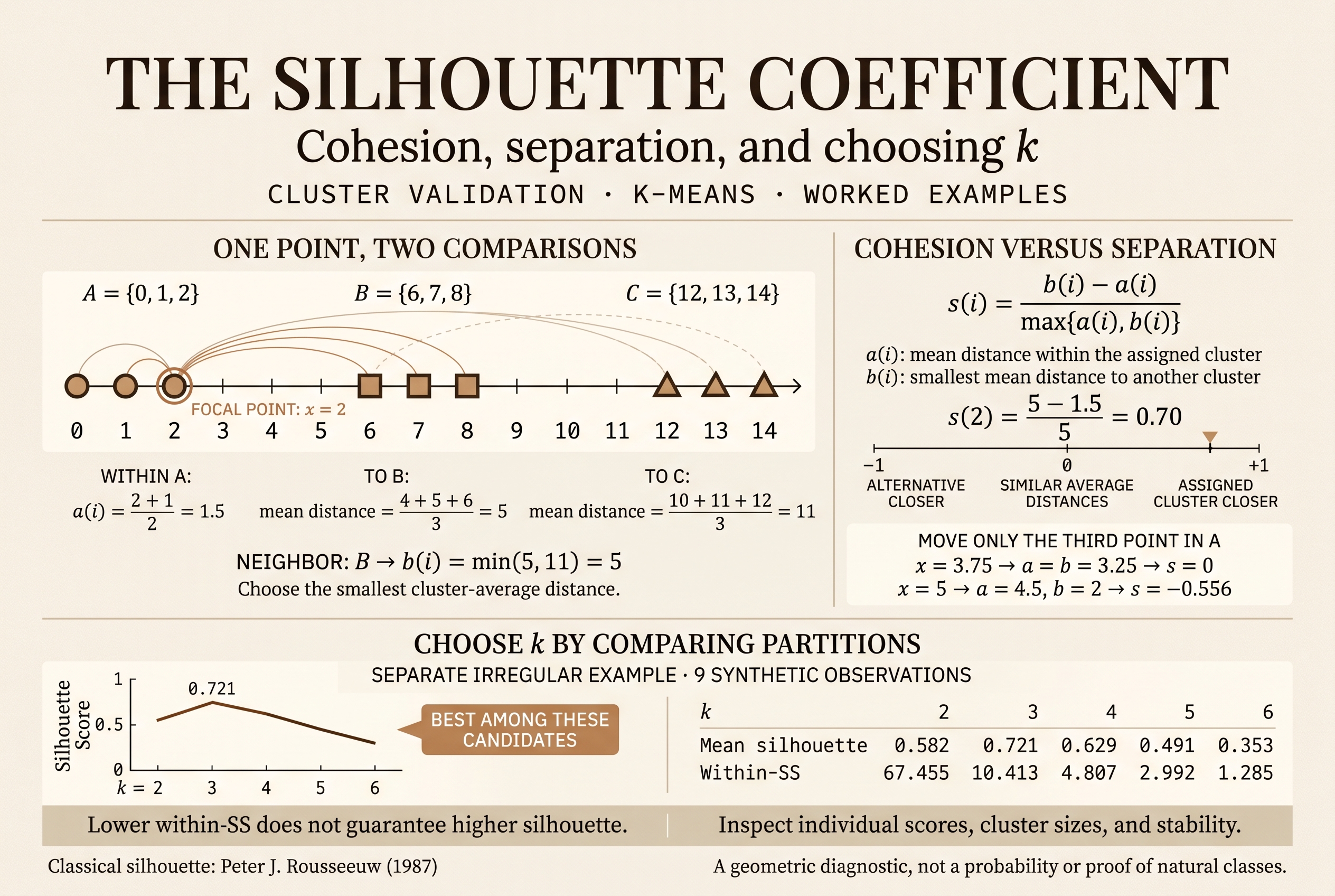
Consider nine one-dimensional observations and a fixed partition: A = {0, 1, 2}, B = {6, 7, 8}, and C = {12, 13, 14}. These are synthetic data with no empirical interpretation attached. We use d(i, j) = |xi − xj|.
For x = 2, the assigned cluster is A. The table contains every relevant distance:
| Destination | Observations | Distances from x = 2 | Average |
|---|---|---|---|
| A, excluding itself | 0, 1 | 2, 1 | a(i) = (2 + 1)/2 = 1.5 |
| B | 6, 7, 8 | 4, 5, 6 | d̄(i, B) = 15/3 = 5 |
| C | 12, 13, 14 | 10, 11, 12 | d̄(i, C) = 33/3 = 11 |
The observation has lower average dissimilarity to its assigned cluster than to B, the closest alternative. The score 0.70 expresses that normalized relationship; it is neither a membership probability nor an accuracy of 70%.
How zero and negative scores arise
Now change only the third point in A: A = {0, 1, t}. B and C retain their values. Each row below represents a different modified dataset, with labels held fixed:
| t | a(t) | b(t) | s(t) |
|---|---|---|---|
| 2 | 1.5 | 5 | 0.700000 |
| 3.75 | 3.25 | 3.25 | 0.000000 |
| 5 | 4.5 | 2 | −0.555556 |
At t = 3.75, the two relevant average dissimilarities are equal. At t = 5, B is closer on average than A. These cases diagnose specified partitions; they are not presented as outcomes of refitting k-means.
05. Individual, cluster-level, and overall interpretation
An s(i) close to 1 indicates high relative cohesion compared with the neighboring cluster; around zero, the average dissimilarities are similar; a negative score indicates that the alternative is closer on average. These readings depend on the data, features, and chosen dissimilarity.
A negative silhouette invites closer examination. It does not, by itself, prove a programming error or require reassignment: the k-means objective and the silhouette criterion differ. Nor does it establish that the observation is an outlier.
The overall mean weights each cluster by its size. Taking an unweighted average of cluster means answers another question and agrees with the overall mean only in particular cases, such as equally sized clusters.
| x | Cluster | a(i) | b(i) | s(i) |
|---|---|---|---|---|
| 0 | A | 1.5 | 7.0 | 0.785714 |
| 1 | A | 1.0 | 6.0 | 0.833333 |
| 2 | A | 1.5 | 5.0 | 0.700000 |
| 6 | B | 1.5 | 5.0 | 0.700000 |
| 7 | B | 1.0 | 6.0 | 0.833333 |
| 8 | B | 1.5 | 5.0 | 0.700000 |
| 12 | C | 1.5 | 5.0 | 0.700000 |
| 13 | C | 1.0 | 6.0 | 0.833333 |
| 14 | C | 1.5 | 7.0 | 0.785714 |
The cluster means are s̄A = 0.773016, s̄B = 0.744444, and s̄C = 0.773016. Because each cluster contains three observations, s̄ = 481/630 ≈ 0.763492.
Read the plot by examining bar lengths, negative scores, cluster sizes, and differences between clusters. The display reveals the distribution summarized by a single mean (Rousseeuw, 1987).
06. Comparing k without treating the maximum as truth
For a candidate set K, one can select the partition with the largest mean silhouette:
This selection is relative to K, the data, preprocessing, and fitting procedure. It neither confirms that clusters exist nor assesses k = 1. When several solutions score similarly, retain them for graphical and substantive examination.
To avoid the symmetric ties in the hand-worked example, now use a different synthetic dataset: {0, 0.8, 2, 6, 7.3, 8, 12, 13.2, 15.5}. All values share one unit. The table reports solutions minimizing W(k) for this small one-dimensional problem; the code includes an exhaustive check over contiguous partitions.
| k | W(k) | Mean silhouette | Minimum size | Singleton clusters |
|---|---|---|---|---|
| 2 | 67.455000 | 0.582098 | 3 | 0 |
| 3 | 10.413333 | 0.721211 | 3 | 0 |
| 4 | 4.806667 | 0.628661 | 1 | 1 |
| 5 | 2.991667 | 0.491256 | 1 | 2 |
| 6 | 1.285000 | 0.353364 | 1 | 3 |
For k = 3, the clusters are {0, 0.8, 2}, {6, 7.3, 8}, and {12, 13.2, 15.5}. Here, further reductions in W(k) from splitting the data are not accompanied by higher silhouettes. Singleton clusters in later solutions contribute zero silhouette by convention.
| Criterion | What it examines | How to use it |
|---|---|---|
| Elbow in W(k) | Marginal improvement as the number of centroids increases. | Look for slope changes; a distinct elbow may be absent. |
| Silhouette | Relative cohesion against the best alternative cluster. | Compare means and within-cluster distributions. |
| Initialization sensitivity | Variation when random seeds change. | Repeat complete fits while keeping preprocessing fixed. |
| Sampling stability and interpretation | Persistence and relevance of clusters for the problem. | Examine resampling, profiles, and domain knowledge. |
These criteria provide complementary evidence. Sensitivity to the seed and stability under changes to the sample are different properties: repeating random seeds does not estimate sampling uncertainty.
07. A reproducible, audited implementation in R
The following script contains the data, an independent implementation of the formula, checks of the hand-worked example, fitting with multiple initializations, and comparison of k = 2, …, 6. For each k, kmeans() retains the best fit according to within-cluster sum of squares, not silhouette (R Documentation, n.d.-b).
The code also checks the minimum sum of squares by enumeration for this small univariate case. That audit exploits n = 9 and the ordered line; it should not be generalized into an efficient strategy for large multivariate problems. Numerical cluster labels can be permuted without changing the partition.
# Silhouette coefficient: worked examples and k-means comparison
# Original article: 2022-04-21 | Revision: 2026-11-11
# Dependency: install.packages("cluster") if it is not already available.
if (!requireNamespace("cluster", quietly = TRUE)) {
  stop('Install the cluster package first: install.packages("cluster")')
}

# Independent calculation from a complete dissimilarity matrix.
silhouette_manual <- function(labels, D) {
  D <- as.matrix(D)
  n <- length(labels)
  stopifnot(n >= 3L, !anyNA(labels), is.numeric(D),
            all(dim(D) == c(n, n)), all(is.finite(D)),
            all(D >= 0), max(abs(D - t(D))) < 1e-10,
            max(abs(diag(D))) < 1e-10)
  groups <- unique(labels)
  stopifnot(length(groups) >= 2L, length(groups) <= n - 1L)
  s <- numeric(n)
  for (i in seq_len(n)) {
    own <- which(labels == labels[i])
    if (length(own) == 1L) {
      s[i] <- 0
      next
    }
    a <- mean(D[i, setdiff(own, i)])
    other <- groups[groups != labels[i]]
    means <- vapply(other, function(g) mean(D[i, labels == g]), numeric(1))
    b <- min(means)
    s[i] <- if (max(a, b) == 0) 0 else (b - a) / max(a, b)
  }
  s
}

# 1. Exact hand-worked example; distances are absolute differences.
x_hand <- matrix(c(0, 1, 2, 6, 7, 8, 12, 13, 14), ncol = 1)
labels_hand <- rep(1:3, each = 3)
D_hand <- dist(x_hand, method = "euclidean")
s_hand <- cluster::silhouette(labels_hand, D_hand)
stopifnot(max(abs(silhouette_manual(labels_hand, D_hand) -
                  s_hand[, "sil_width"])) < 1e-12,
          abs(s_hand[3, "sil_width"] - 0.7) < 1e-12,
          abs(mean(s_hand[, "sil_width"]) - 481 / 630) < 1e-12)
print(data.frame(x = x_hand[, 1], cluster = labels_hand,
                 silhouette = round(s_hand[, "sil_width"], 6)))

# Moving only the third point creates positive, zero and negative examples.
for (t in c(2, 3.75, 5)) {
  xt <- x_hand
  xt[3, 1] <- t
  actual <- cluster::silhouette(labels_hand, dist(xt))[3, "sil_width"]
  a <- mean(abs(t - c(0, 1)))
  b <- min(mean(abs(t - c(6, 7, 8))), mean(abs(t - c(12, 13, 14))))
  expected <- (b - a) / max(a, b)
  stopifnot(abs(actual - expected) < 1e-12)
  cat(sprintf("t = %.2f; a = %.2f; b = %.2f; s = %.6f\n", t, a, b, actual))
}

# Check singleton, coincident-point and zero-denominator conventions.
for (case in list(
  list(x = c(0, 1, 10), labels = c(1L, 1L, 2L)),
  list(x = c(0, 0, 0, 0), labels = c(1L, 1L, 2L, 2L)),
  list(x = c(0, 0, 10, 10), labels = c(1L, 1L, 2L, 2L))
)) {
  dd <- dist(matrix(case$x, ncol = 1))
  reference <- cluster::silhouette(case$labels, dd)[, "sil_width"]
  stopifnot(all(is.finite(reference)),
            max(abs(silhouette_manual(case$labels, dd) - reference)) < 1e-12)
}

# 2. Irregular synthetic data: avoids the ties of the hand-worked example.
x <- matrix(c(0, 0.8, 2, 6, 7.3, 8, 12, 13.2, 15.5), ncol = 1,
            dimnames = list(paste0("P", 1:9), "x"))
stopifnot(is.numeric(x), all(is.finite(x)), nrow(unique(x)) >= 6L)
# All observations use one common unit. No scaling is needed here.
# For multivariate data, justify feature selection and scaling before fitting.
# x <- scale(x)  # Optional; do not standardize constant columns.
D <- dist(x, method = "euclidean")
ks <- 2:6
models <- vector("list", length(ks))
silhouettes <- vector("list", length(ks))
rows <- vector("list", length(ks))
for (j in seq_along(ks)) {
  k <- ks[j]
  set.seed(20220421L + k)
  fit <- kmeans(x, centers = k, nstart = 100, iter.max = 100,
                algorithm = "Hartigan-Wong")
  if (!is.null(fit$ifault) && fit$ifault != 0L) stop("k-means did not converge")
  s <- cluster::silhouette(fit$cluster, D)
  stopifnot(max(abs(silhouette_manual(fit$cluster, D) -
                    s[, "sil_width"])) < 1e-12)
  models[[j]] <- fit
  silhouettes[[j]] <- s
  rows[[j]] <- data.frame(k = k, within_ss = fit$tot.withinss,
                          mean_silhouette = mean(s[, "sil_width"]),
                          negative_fraction = mean(s[, "sil_width"] < 0),
                          smallest_cluster = min(fit$size),
                          singleton_clusters = sum(fit$size == 1L))
}
results <- do.call(rbind, rows)
print(results, digits = 7, row.names = FALSE)
best <- which.max(results$mean_silhouette)
cat("Selected k among the candidates:", results$k[best], "\n")
print(summary(silhouettes[[best]]))

# Audit the small ONE-DIMENSIONAL example against all contiguous partitions.
# This is feasible only because n = 9; it is not a general-purpose workflow.
# For sorted univariate squared-error k-means, a global optimum is contiguous.
x_sorted <- sort(x[, 1])
exact_sse <- vapply(ks, function(k) {
  cuts <- combn(seq_len(length(x_sorted) - 1L), k - 1L)
  min(apply(cuts, 2, function(cut) {
    starts <- c(1L, cut + 1L)
    ends <- c(cut, length(x_sorted))
    sum(vapply(seq_len(k), function(g) {
      z <- x_sorted[starts[g]:ends[g]]
      sum((z - mean(z))^2)
    }, numeric(1)))
  }))
}, numeric(1))
stopifnot(max(abs(results$within_ss - exact_sse)) < 1e-10,
          results$k[best] == 3L,
          abs(results$mean_silhouette[best] - 0.7212109713028838) < 1e-12)

# 3. Repeat the entire fitting procedure with different seeds.
# These ranges describe initialization sensitivity, not sampling uncertainty.
seeds <- 1:20
stability <- do.call(rbind, lapply(ks, function(k) {
  means <- vapply(seeds, function(seed) {
    set.seed(seed)
    fit <- kmeans(x, centers = k, nstart = 100, iter.max = 100)
    mean(cluster::silhouette(fit$cluster, D)[, "sil_width"])
  }, numeric(1))
  data.frame(k = k, minimum = min(means), median = median(means),
             maximum = max(means))
}))
print(stability, digits = 7, row.names = FALSE)

# 4. Export the complete analysis to the current working directory.
write.csv(results, "silhouette_k_comparison.csv", row.names = FALSE)
write.csv(stability, "silhouette_initialization_sensitivity.csv", row.names = FALSE)
write.csv(data.frame(id = rownames(x), x = x[, 1],
                     cluster = models[[best]]$cluster,
                     silhouette = silhouettes[[best]][, "sil_width"]),
          "silhouette_individual_results.csv", row.names = FALSE)
paper <- "#fffdf7"
ink <- "#2c2418"
copper <- "#8b4513"
pdf("silhouette_diagnostics.pdf", width = 7, height = 6, bg = paper)
par(col = ink, col.axis = ink, col.lab = ink, col.main = ink,
    fg = ink, bg = paper)
plot(results$k, results$mean_silhouette, type = "b", pch = 19,
     col = copper, xlab = "Number of clusters (k)",
     ylab = "Mean silhouette", ylim = c(0, 1))
plot(silhouettes[[best]], col = copper, border = NA,
     main = paste("Silhouette | k =", results$k[best]))
abline(v = results$mean_silhouette[best], lty = 2, col = ink)
plot(results$k, results$within_ss, type = "b", pch = 19,
     col = copper, xlab = "Number of clusters (k)",
     ylab = "Within-cluster sum of squares")
dev.off()
writeLines(capture.output(sessionInfo()), "silhouette_session_info.txt")
In addition to the displayed tables, the script writes three CSV files, a PDF containing diagnostic plots, and a session-information file. Files are created in R’s current working directory. The twenty-seed repetition describes initialization sensitivity in this example; it is not a confidence interval.
08. Limitations and choices that must be reported
The silhouette tends to favor convex, separated clusters under the chosen geometry. Elongated, chained, or density-defined structures may score poorly even when they matter for the problem. Comparing algorithms therefore requires a shared interpretation of what constitutes a cluster (scikit-learn developers, n.d.).
- Features and scales. Units and weights change dissimilarities. Standardization is an analytical choice, not an automatic correction appropriate for every problem.
- Outliers and unequal sizes. Examine their effect on averages and small clusters. Report cluster means, sizes, and problematic observations alongside the overall mean.
- High dimensionality. Assess whether the selected distances retain useful contrasts. A projection used for visualization does not replace the geometry used to fit and evaluate the model.
- Candidates and comparability. Use the same observations and dissimilarity for a direct comparison; document any changes.
- Computational cost. A full distance matrix requires memory of order n². Sampling can reduce the diagnostic cost, but specify whether averages use only the subsample or all observations as references.
- Absence of structure. Examine suitable reference scenarios or stability before assigning meaning to a maximum. An available partition is not equivalent to confirmed empirical structure.
When using resampling, describe observation selection, refitting, and the comparison between partitions. Cluster labels are arbitrary: directly comparing their numerical values does not measure stability.
09. Mathematical note: cluster geometry and topology
This revision preserves the mathematical interest of Nabi (2022) while clarifying its vocabulary. Similar terminology does not justify identifying different definitions.
| In clustering | In topology or algebra | Necessary distinction |
|---|---|---|
| Geometric cohesion or compactness | Compactness: every open cover has a finite subcover. | Every finite set is compact, even when its points are far apart. |
| Separation between clusters | Separability: existence of a countable dense subset. | It does not quantify between-cluster distance; ℝᵖ is separable in its usual topology. |
| Neighborhood connectivity | Connectedness: absence of a separation into disjoint nonempty relatively open sets. | A neighbor graph and the topology of the observed point set are different constructions. |
| A subset of observations | Vector subspace: contains zero and is closed under addition and scalar multiplication. | An arbitrary cluster of observations need not satisfy these conditions. |
Two examples make the difference explicit. {0, 1} and {0, 1000} are compact subsets of ℝ, although their diameters are 1 and 1000. Every finite set of distinct points in ℝᵖ also has the discrete relative topology: a sufficiently small ball isolates each point. With more than one point, the set is disconnected even when it looks like a very tight cloud.
For a subset C of a topological space, a relevant separation would be C = U ∪ V, where U and V are nonempty, disjoint, relatively open subsets of C: U ∩ V = ∅. Their union reconstructs C; their intersection records shared elements. C is connected when no such separation exists.
An open Euclidean ball contains points whose distance from its center is less than its radius; the sphere consists of points at exactly that distance. Neither definition alone turns a statistical cluster into a connected region.
These distinctions use definitions of metric spaces and compactness ({cite(‘lebl’,’Lebl, n.d.’)}). Rigorous links to topology require explicitly defining an additional structure, such as a graph or a union of balls, and then studying its properties.
10. How to report the result
A useful report identifies the data and features, preprocessing, algorithm and options, evaluation dissimilarity, candidate values of k, and sensitivity of the result. It accompanies the overall mean with cluster sizes and cluster-level diagnostics.
For nine synthetic one-dimensional observations, k = 2, …, 6 were compared using k-means and Euclidean distance. The largest mean silhouette among the candidates was 0.721211 at k = 3. This choice was interpreted alongside within-cluster sum of squares, cluster sizes, and individual diagnostics.
The conclusion states which evidence supports the selected solution and under what conditions. Its ultimate usefulness depends on whether the clusters help answer the research question.
11. References
- Hartigan, J. A., & Wong, M. A. (1979). Algorithm AS 136: A k-means clustering algorithm. Journal of the Royal Statistical Society. Series C (Applied Statistics), 28(1), 100–108. https://doi.org/10.2307/2346830
- Lebl, J. (n.d.). Basic analysis: Introduction to real analysis (Vol. II). Retrieved November 11, 2026, from https://www.jirka.org/ra/
- Nabi, I. (2022). Construcción e interpretación del coeficiente silueta en agrupamientos por k-medias. Marxist Philosophy of Science. https://marxistphilosophyofscience.com/wp-content/uploads/2022/04/construccion-e-interpretacion-del-coeficiente-silueta-en-agrupamientos-por-k-medias-isadore-nabi-1.pdf
- R Documentation. (n.d.-a). Compute or extract silhouette information from clustering [Software documentation]. Retrieved November 11, 2026, from https://stat.ethz.ch/R-manual/R-patched/library/cluster/html/silhouette.html
- R Documentation. (n.d.-b). K-means clustering [Software documentation]. Retrieved November 11, 2026, from https://stat.ethz.ch/R-manual/R-patched/library/stats/html/kmeans.html
- Rousseeuw, P. J. (1987). Silhouettes: A graphical aid to the interpretation and validation of cluster analysis. Journal of Computational and Applied Mathematics, 20, 53–65. https://doi.org/10.1016/0377-0427(87)90125-7
- scikit-learn developers. (n.d.). Clustering [Software documentation]. Retrieved November 11, 2026, from https://scikit-learn.org/stable/modules/clustering.html
Leave a Comment/Deja un Comentario