Political Economy and Probability Theory: Marx, Adam Smith, and the Law of Large Numbers

Do All Workers Get Exploited the Same?
Testing a Marxian Assumption with Probability Theory

How sixty years of U.S. sectoral data and non-classical laws of large numbers were used to examine a foundational assumption behind the Marxian average rate of profit

Based on: Gómez Julián, J. M. (2022). Ciencia Económica, 11(17), UNAM

~ 9 min read

A consequential assumption sits behind Marxian analyses of the average rate of profit whenever differences in the degree of labor exploitation across productive sectors are not explicitly modeled: sectoral rates of surplus value may be treated as tending toward uniformity. Adam Smith supplied the original economic argument for such a tendency, and within Marxian political economy the proposition acquired central importance. But can that tendency be defended when actual sectors are neither independent nor statistically identical? A 2022 paper by José Mauricio Gómez Julián in Ciencia Económica approaches the question from three directions at once: probability theory, the concrete labor-market mechanisms discussed by Smith and Marx, and statistical evidence from the United States between 1960 and 2020.

The Problem, in Plain Language

In Marxian theory, surplus value is the value produced by labor beyond the value represented by labor-power. Empirically, the paper approximates the rate of surplus value using modern national accounts: gross operating surplus is taken as a representation of surplus labor time and employee compensation as a representation of necessary labor time. Their ratio provides the sectoral rate used in the statistical analysis.

The issue matters because the tendency toward uniform sectoral rates of surplus value is part of the foundation on which the formation of an average rate of profit and, consequently, Marxian prices of production rests. But an important nuance is easily lost here. The paper does not treat prices of production as pre-existing equilibrium prices around which market prices merely oscillate. Drawing on Carchedi and de Haan, it emphasizes a dynamic interpretation: market prices exist first, and capitalist competition — including technological competition and movements of capital — pressures them toward a systemic average. Prices of production exist through this very process of convergence rather than as a fixed center established in advance.

The empirical question is therefore not whether every industry displays exactly the same exploitation rate at every instant. The proposition under examination is a tendency toward asymptotic uniformity: as the analysis approaches a sufficiently long period and/or a sufficiently large collection of relevant sectors, do sectoral rates behave in a way consistent with convergence toward a global expected value?

Why the Asymptotic Perspective Matters

The paper connects this question to Marx’s theory of knowledge. Its argument is that Marx’s method cannot be reduced to the passive acceptance of isolated empirical facts. Through a materialist appropriation of Hegelian dialectics, the analysis privileges totality: the phenomenon must be understood through its relations, its development, and the larger system of which it forms a part. In the paper, the term asymptotic regime condenses this idea statistically — a sufficiently long time horizon, a sufficiently large number of units, or both.

This matters because a sector observed in isolation may differ substantially from another sector. Uniformity, if it exists, need not appear as point-by-point equality. It may instead be a property that becomes visible only when the system is considered on a sufficiently large scale.

Enter the Law of Large Numbers

The mathematical framework is the Law of Large Numbers (LLN). In broad terms, laws of large numbers describe conditions under which averages stabilize around an expected value as the amount of information grows. The strong version concerns almost-sure convergence; the weak version concerns convergence in probability.

The difficulty is immediate. Classical formulations typically rely on strong assumptions such as independence and identical distribution. Those conditions are not realistic for capitalist sectors. Industries interact through production chains, competition, wages, technology, demand, and capital movements; and their productive structures differ. The paper’s own statistical results confirm that the sectoral variables are neither identically distributed nor, in general, linearly independent.

That does not make the LLN irrelevant. Rather, the theoretical part of the paper asks whether more general versions of the law can accommodate the structure of the economic problem. The answer is qualified: several mathematical results relax different parts of the classical assumptions, but they do not all do so in the same way.

What the Mathematical Literature Actually Establishes

Li, Rao and Wang (1995): study a strong law for weighted sums of independent random variables with multidimensional indices under specific structural and moment conditions.
Adler and Rosalsky (1987): establish a strong-law result for normalized weighted sums of independent and identically distributed random variables.
Chen and Sung (2016): generalize weighted-sum results under stochastic-dominance and weighting conditions, relaxing restrictions relevant to the distributional structure.
Sung (2011): is especially important for the economic application because it provides sufficient conditions under which the variables may be dependent, subject to moment and other technical requirements.
Andrews (1988) and Davidson (2021): provide weak-law results and a broader framework for weakly dependent processes, including mixingale-type structures relevant to econometrics.

“Smith’s proposition concerning the law of tendency toward uniformity is consistent with the logic behind certain varieties of the Law of Large Numbers.” Translation of the paper’s conclusion — Gómez Julián, 2022

The word certain is essential. The paper does not claim that simply invoking a non-classical LLN automatically proves the Marxian proposition. Formal consistency depends on satisfying the conditions of the particular theorem being used. In some cases this may require transformations of the dataset — for example, grouping or disaggregating sectors, arranging observations in structures such as triangular arrays, or estimating missing periods where appropriate. Whether such requirements can actually be met depends on the concrete dataset.

What Counts as a Productive Sector?

Before performing the statistical analysis, the paper faces a specifically Marxian classification problem: not every activity appearing in national accounts necessarily belongs in the calculation of the average rate of profit. The relevant sectors are those treated as productive in relation to the circuit of capital and the production of surplus value.

This is particularly important for services. Drawing on the literature on productive and unproductive labor, the study distinguishes activities that directly produce surplus value, activities that facilitate its production elsewhere, and activities outside the relevant circuit of capital. After harmonizing sector classifications across the historical period and applying those theoretical criteria, the empirical analysis works with 36 productive sectors.

What the U.S. Data Show

The empirical component uses data from the U.S. Bureau of Economic Analysis for the period 1960–2020. Sectoral rates of surplus value are constructed from gross operating surplus and employee compensation, and the study then examines probability distributions, pairwise Pearson correlations, and the differences between sectoral location measures and their global counterparts.

Key Empirical Findings

The sectors are not identically distributed: among the 36 sectors, 16 are best fitted by a Uniform distribution, 13 by Cauchy, 3 by Logistic, 2 by Log-Normal, and 2 by Weibull. None is best described by a Normal distribution.
The sectors are not generally linearly independent: 630 pairwise Pearson correlations are calculated. Their mean is approximately 0.081 and their median approximately 0.140.
Substantial pairwise dependence is not rare: 256 of the 630 correlations — about 40.63% — are at least 0.30. The paper therefore rejects the idea that the sectors can generally be treated as linearly independent.
Most summary measures of the differences are close to zero: relative to the global mean, the sum of sectoral differences is approximately 3.38 × 10⁻¹⁴ and their mean approximately 9.38 × 10⁻¹⁶. Relative to the global median, the corresponding values are also small.
There is an important exception: the median of the differences calculated relative to the global mean is not close to zero. The paper therefore describes the evidence as a tendency toward reciprocal nullification in general, not as perfect cancellation in every statistic.
The differences have different distributional forms: those calculated relative to the global mean are best fitted by a Cauchy distribution, with Logistic as the second-best option; those relative to the global median are best fitted by a Uniform distribution, with Normal as the second-best option.

This pattern is important precisely because the empirical data do not reproduce the assumptions of the classical LLN. The sectors remain heterogeneous and interconnected. Yet the descriptive behavior of their deviations provides evidence, in the author’s interpretation, in favor of a tendency toward reciprocal nullification when the system is considered as a whole.

Why Conventional Significance Tests Were Set Aside

The paper originally considers tests for differences between sectoral means or medians and their global counterparts, including Student’s t procedures and Wilcoxon procedures, together with bootstrapping. It ultimately argues that the available inferential tests are not appropriate for drawing valid conclusions from this particular structure of data.

The problem is not simply non-normality. Depending on the procedure, assumptions concerning distributional form, linear independence, pairing, and equal sample sizes become relevant. The economic variables are interdependent by construction, and bootstrapping does not solve the entire difficulty: although resampling can break the relation between the immediately compared groups, it does not eliminate dependence among the sectoral components that make up the global group.

An especially important nuance is that the discarded tests did indicate statistically significant differences. The paper nevertheless refuses to treat those results as valid inferential evidence because the required conditions are not adequately satisfied. It therefore replaces that inferential route with a descriptive — or, as the paper itself suggests, perhaps more accurately semi-descriptive — analysis based on the behavior and probability distributions of the differences.

Smith, Marx, and the Economic Mechanism

The probability argument is only one dimension of the paper. A second dimension returns to Adam Smith’s account of labor-market adjustment. Smith argues that the total advantages and disadvantages of different employments in the same locality must either be equal or continually tend toward equality; otherwise workers and capital would move in ways that erode unusually favorable or unfavorable conditions.

The paper organizes Smith’s discussion around seven factors affecting compensation: the simplicity or difficulty of the work; whether it is pleasant or unpleasant; danger and effects on health; regularity or temporariness of employment; the degree of trust placed in the worker; the probability of professional success; and subjective considerations such as passion for an occupation, reputation, confidence in one’s abilities, and confidence in one’s luck.

These factors matter because they do not imply isolated sectors. Quite the opposite: sectoral rates can be linked directly through the organic interdependence of capitalist production and indirectly through common forces affecting wages and working conditions. In this sense, the economic mechanism described by Smith and Marx is more naturally compatible with generalized probabilistic frameworks that permit dependence than with a classical model requiring reciprocal independence.

• • •

So What Does the Paper Actually Establish?

The conclusion is favorable to the uniformity hypothesis, but it is carefully delimited. At the theoretical level, the logic of Smith’s tendency toward uniform sectoral rates of surplus value is consistent with certain strong and weak versions of the Law of Large Numbers that allow correlated variables and/or do not require identical distributions. This formal consistency is conditional on the concrete requirements of the relevant mathematical results being satisfiable.

At the empirical level, the U.S. data show precisely the heterogeneity and interdependence that rule out a simplistic classical-LLN argument. At the same time, the descriptive analysis of sectoral deviations produces results that point in a direction favorable to Smith and Marx’s proposition that sectoral rates tend toward uniformity.

This is therefore not a demonstration that every capitalist economy, in every historical period, must exhibit a uniform rate of surplus value. Nor does the study claim that all sectors possess the same rate at each moment. Its narrower and more defensible conclusion is that the assumption used in long-run Marxian analyses of the average rate of profit has both a plausible probabilistic formulation and empirical evidence in its favor for the U.S. case examined.

That distinction matters. The paper’s contribution is not to eliminate sectoral diversity, but to ask whether diversity at the level of the parts can coexist with an asymptotic regularity at the level of the whole. Its answer is cautiously affirmative — and it is precisely the combination of heterogeneity, interdependence, and systemic regularity that makes the problem mathematically and economically interesting.

15 July, 2026

bayesianOU: Exploring Market Price Gravitation via Ornstein-Uhlenbeck Process

You can also find this library at CRAN and download it directly from R and RStudio.

LISTEN TO THIS POST AS A PODCAST:

When Market Prices Gravitate: A Bayesian Look at an Old Question in Economics

An old question, asked again — properly

There is a question in economics that is older than most of the academic disciplines that border it. Do market prices — the noisy, day-to-day, here-and-now prices at which goods actually change hands — tend to settle toward some underlying center of gravity? And if they do, how fast, how violently, and through what mechanism?

Classical political economy, from Smith and Ricardo through Marx, thought they do. The idea was that behind the churning surface of market prices there sit “prices of production”: long-run, cost-anchored prices toward which actual prices are pulled, the way a spring pulls a weight back toward its rest position. In the Marxian version, there is one more layer underneath: those prices of production themselves are supposed to gravitate around “values,” the labour embodied in commodities. Whether any of this is true is an empirical question, and for a long time the empirical tools to answer it were not really up to the job.

A small R package called bayesianOU, written by José Mauricio Gómez Julián and hosted on GitHub, takes a serious swing at that question. It is not the first attempt to test price gravitation statistically, but it is one of the most technically careful I have seen, and it is built in a way that is instructive far beyond the Marxian debate that motivates it. What follows is a walkthrough of what the package does, why it is interesting, and — just as importantly — where it honestly admits its own limits.

The tool that makes it possible: the Ornstein-Uhlenbeck process

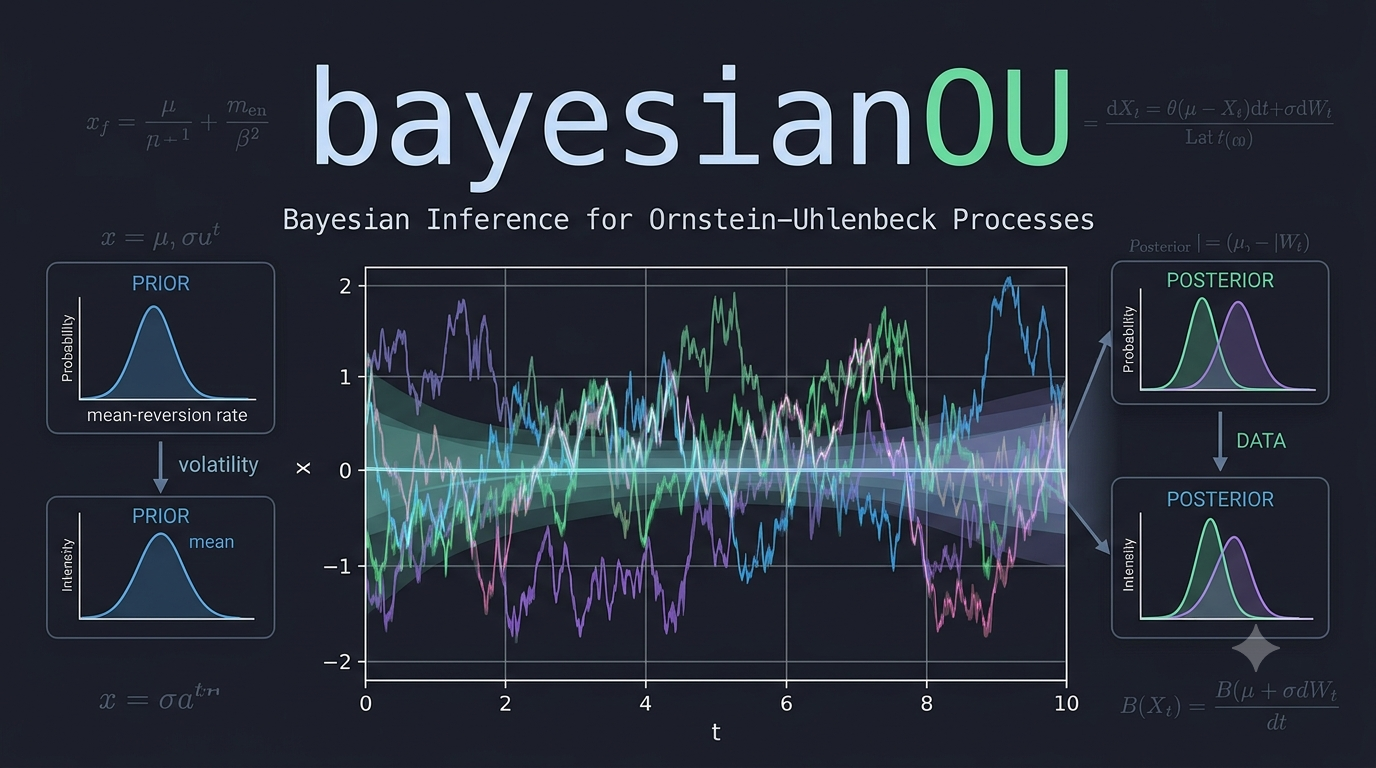
Strip the economics away for a moment and the statistical core of the package is a workhorse object from physics: the Ornstein-Uhlenbeck (OU) process. Imagine a particle moving in a fluid, attached to a spring. Brownian motion jiggles it randomly; the spring pulls it back toward a fixed point. The further it drifts away, the harder the pull. The result is a wiggly series that never settles but always tends to settle — a mean-reverting random walk.

The OU process is exactly the mathematical object you want when you suspect a variable is noisy but anchored. It has a “speed of reversion” (how hard the spring pulls) and an “equilibrium level” (where the spring’s rest point is). Estimate those, and you can say something quantitative about gravitation: not just “yes, prices come back,” but “they come back with a half-life of about nine years.”

That number — the half-life — is the prize. It is the difference between “market prices eventually settle” (which could mean anything) and “market prices settle on a timescale comparable to a business cycle” (which is a falsifiable, interpretable claim).

What the package actually builds

The package fits, by Bayesian inference, a family of models built on the OU process but considerably richer than the textbook version. There are two first-class models, sharing one inference engine.

The single-level model

The first model asks: do market prices revert toward an equilibrium that is a function of the prices of production, and what does that reversion look like once we let it be nonlinear, volatile, heavy-tailed, and structurally heterogeneous across sectors?

Each of those adjectives is doing real work, and each corresponds to a feature that simpler approaches handle poorly or not at all:

Nonlinear drift. A plain OU process pulls back with a force proportional to the deviation. The package allows a cubic correction, so the restoring force can strengthen super-linearly when prices are far from equilibrium. This matters: real markets may behave gently near the center and violently at the extremes, and a linear model cannot represent that.
Stochastic volatility. Financial data, and economic data generally, go through quiet stretches and turbulent ones. The package does not assume a single noise level; it lets the volatility itself wander over time, following its own mean-reverting process on the log-variance. This is the same idea that powers modern stochastic-volatility models in finance, and it is essential for not fooling yourself about the precision of your estimates.
Heavy tails. Economic shocks are not Gaussian. Crashes, booms, and policy shocks produce outliers that a normal distribution would call essentially impossible. The package uses Student-t innovations and estimates the degrees of freedom from the data, so the model can discover for itself just how fat-tailed the world is.
Hierarchical structure across sectors. An economy has dozens of sectors, and each one presumably has its own reversion speed, its own equilibrium, its own noise. Estimating each sector in isolation throws away the information that they are all part of the same economy. Estimating them all with one set of parameters pretends they are identical. The package takes the middle path — hierarchical, or “partial pooling,” priors — where each sector’s parameters are drawn from a shared distribution whose properties the model also estimates. Sectors borrow strength from one another without being forced into lockstep.
A time-varying coupling. This is the most economically loaded feature. The strength with which market prices track prices of production is allowed to depend on the aggregate profit rate (what the package calls TMG). When the general rate of profit is high, the pull of production prices on market prices may be one thing; when it is low, another. Whether that modulation exists, and in which direction, is a hypothesis the model can test rather than assume.

All of this is estimated jointly, with full Bayesian uncertainty, using Stan’s Hamiltonian Monte Carlo sampler. You do not get a point estimate of the reversion speed; you get a posterior distribution, and from it a credible interval and a probability statement like “there is a 95% chance the half-life is between six and eighteen years.”

The nested cascade

The second model is the more ambitious one, and it is where the package earns its “nested” branding. Instead of market prices reverting to a fixed equilibrium, they revert to a latent production price — a hidden, unobserved series that itself evolves over time according to its own OU process, driven by the general profit rate. And, if you turn on the third level, that latent production price in turn gravitates around an observed “value” index built directly from labour-content accounting.

So the full structure is a cascade: market price → latent production price → value. Each arrow is an OU reversion, each with its own speed, and the speeds are constrained so that the outer (market) layer reverts faster than the inner (production) layer — an economically natural separation of timescales, enforced softly so the data can push back.

The reason this matters is that it converts a slogan — “prices of production gravitate around values” — into a literal statistical hierarchy that can be fit to data and compared against alternatives. The headline empirical result, from a fit to 37 US sectors over 1960–2020, is a value-coupling coefficient essentially equal to one, with the posterior probability of it being positive effectively equal to one. In plain terms: in standardized units, prices of production track labour values almost one-for-one. That is a found result, not an assumed one — the prior on the coupling was centred at zero, deliberately neutral.

The inference engine, and why it is not a footnote

It would be easy to glance at the model description, nod, and move on. But how these quantities are estimated is half of what makes the package serious, and it is worth a paragraph for readers who do not think about MCMC every day.

Bayesian inference works by exploring the space of all parameter values consistent with both the data and the prior, and characterizing that space as a probability distribution. For models this complex — with latent volatility paths, hierarchical structure, and hundreds of parameters — you cannot do that with pencil and paper. You use a Markov chain Monte Carlo sampler, specifically Hamiltonian Monte Carlo, which borrows an idea from physics: give the parameter space a “potential energy” (the log-posterior) and a “kinetic energy” (a randomly chosen momentum), and let the system glide around the posterior like a ball rolling over a landscape.

Stan’s NUTS sampler automates this about as well as it can be automated, and the package uses it with within-chain parallelism (via Stan’s reduce_sum) to handle the fact that the likelihood must be summed over many timepoints and sectors. The diagnostics — R-hat for chain agreement, effective sample size, divergence counts — are surfaced through a validate_ou_fit function, and the package is explicit that you should look at them before believing anything.

Model comparison is done with PSIS-LOO, a clever technique that approximates leave-one-out cross-validation without refitting the model dozens of times, by reweighting the posterior draws using importance sampling. It is the modern standard, and the package is appropriately cautious about it: because the model has a latent volatility state at every observation, plain LOO is known to be optimistic, and the documentation says so plainly.

The honesty that makes it credible

Here is where the package surprised me, and here is why I think it deserves a wider audience than the Marxian-economics niche it lives in.

A naïve reading of the results would be triumphant: the value coupling is one-to-one, the reversion exists, the half-life is about nine years. But the package’s own validation section does something rare. It runs the model against legitimate rivals on genuinely held-out data — a full decade, 2011 to 2020 — and reports, without spin, that a random walk beats the OU model at forecasting, that a no-gravitation restriction ties or beats it, and that the value term adds no detectable predictive density.

That sounds like a refutation. The package argues, carefully, that it is nothing of the sort — and the argument is the most intellectually interesting thing here.

The key move is to distinguish two different questions. One is structural: does a reversion mechanism exist, and how fast is it? The other is predictive: can you forecast next year’s price better than a naïve benchmark? These are related but not identical, and for a slow process they come apart in a specific, predictable way.

If gravitation is real but slow — a half-life of nine years on a dataset whose test window is a decade — then over the forecast horizon the process looks, to first order, like a random walk. The reversion is there, but it is too weak to show up in a one-step or few-step prediction. The random walk, which assumes no reversion, will forecast almost as well, because over short horizons a barely-reverting process and a non-reverting one are nearly indistinguishable. So the random walk winning the forecasting horse race is not evidence against gravitation; it is evidence consistent with gravitation being slow.

This is not special pleading. It is a logical point about what different functionals of a model can and cannot tell you. The structural parameters — estimated from the joint likelihood over the whole panel, borrowing strength across 37 sectors and 61 years — use far more information than any single-series forecast. They can pin down a central tendency that a univariate test cannot. And the package shows, through simulation-based calibration and adversarial negative controls, that the estimation pipeline does not manufacture gravitation when none is present: feed it a true random walk and it reports a half-life of about fifty years; feed it a null value-coupling and the posterior honestly covers zero.

The low-kappa trap, and why it matters to everyone

The package names a difficulty it calls the low-kappa trap, and it is worth understanding because it is a trap that catches far more than Marxian price theory.

Kappa is the reversion speed. As kappa shrinks toward zero, the OU process approaches a pure random walk. The trouble is that there is no bright line separating “slow mean reversion” from “no mean reversion.” It is a continuum, and three distinct problems stack up exactly there:

Algebraically, reversion speed and discrete-time persistence are two sides of the same coin; kappa going to zero is the same as the autocorrelation going to one. There is no internal frontier.
Statistically, the power of a unit-root test — the standard tool for asking “is this a random walk?” — collapses exactly as the truth approaches the random walk boundary. With a finite sample and a half-life comparable to the sample length, the test simply cannot tell. This is a well-known result in econometrics, and it is why decades of “is the real exchange rate stationary?” papers argued past one another.
Numerically, if the reversion speed is parameterized to be strictly positive (as it must be, for the sampler to behave), then “the probability that kappa is greater than zero” is trivially one — it tells you nothing. The informative quantity is the half-life, and the probability that the half-life exceeds some sensible horizon.

The package’s response to the trap is instructive. It does not pretend the trap is not there. It states all three layers explicitly, reports the slow tail honestly (one sector has a non-trivial posterior probability of a half-life beyond forty years), and argues that the joint hierarchical posterior — which pools information across the whole panel — is a more powerful discriminator than any univariate test. That is a defensible position, and it is stated with the caveat attached rather than buried in a footnote.

This is the broader lesson. Anyone working with time series that might be slowly mean-reverting — interest rates, real exchange rates, commodity prices, climate variables, pollutant concentrations — runs into exactly this trap. The package’s framing of it, in three layers, is one of the clearest expositions I have read, and it would travel well into any of those domains.

What I appreciate, and what I would watch for

A few things stand out as genuinely good practice, and they are worth naming because they are rarer than they should be.

The separation of economic and sampler convergence. The package is scrupulous about not confusing two senses of “convergence.” Economic convergence — does the price revert? — is a statement about kappa and the half-life. Sampler convergence — did the MCMC chains agree? — is a statement about R-hat and divergences. These share a word and nothing else, and conflating them is a classic source of muddled reasoning. The documentation keeps them lexically distinct throughout.

Neutral priors on the load-bearing hypotheses. The prior on the profit-rate modulation is centred at zero. The prior on the value coupling is centred at zero. The package does not bake the answer into the question. When the posterior then moves clearly away from zero, that means something.

Out-of-sample integrity by construction. A subtle and common error in time-series work is “leakage”: accidentally letting future information contaminate the training procedure, so that out-of-sample results are secretly in-sample. The package offers a fit_window switch that keeps the two designs genuinely separate, and it computes the common-factor loadings from the training window only. This is the kind of plumbing detail that separates trustworthy work from work that just looks trustworthy.

The negative results are reported. Many packages, and most blog posts about them, would quietly omit the fact that a random walk out-forecasts the model. This one leads with it and then reasons about it. That is how a field accumulates reliable knowledge rather than just encouraging headlines.

What should a careful reader watch for? The half-life estimate of about nine years is, by the package’s own account, probably conservatively slow — a controlled study of the disaggregation step suggests the true figure may be closer to seven or eight. The cubic nonlinearity is a minor refinement on this data (its coefficient sits near its prior). The Student-t degrees of freedom and the stochastic-volatility scale are weakly identified when both are present, a known tension the documentation flags but does not resolve. And the headline value-coupling result, while striking, is measured on standardized levels that share a cost-price component by construction; the package defends this with a “wedge” argument — subtracting the shared component and testing the residual — but a sceptical reader should follow that argument itself rather than take it on trust.

None of these caveats undermine the project. They are the project. A statistical framework that cannot articulate its own soft spots is not a framework you should believe.

Why it is worth your time

You do not need to be a Marxian economist, or any kind of economist, to get something out of this package. If you work with time series that exhibit slow, noisy reversion toward a moving target — and a great deal of the physical and social world does — the modelling ideas here are directly portable: the nonlinear OU drift, the stochastic volatility, the hierarchical pooling across groups, the careful separation of structural estimation from forecasting, and the three-layer diagnosis of the low-reversion trap.

And if you are interested in the classical question of whether prices gravitate toward values, this is about as good a statistical treatment as you will find: modern machinery, honest reporting, and a willingness to let the data argue back against the theory that motivated the exercise in the first place.

The repository, the full mathematical specification, the validation blocks, and a frank discussion of every methodological decision live at github.com/IsadoreNabi/bayesianOU, with the wiki carrying the complete technical detail. Read the methodology notes before you quote a number; that is what they are there for.

13 July, 2026

Revisiting the theory of long depressions BY MICHAEL ROBERTS

Revisiting the theory of long depressions

22 December, 2024

Sectorial Exclusion Criteria in the Marxist Analysis of the Average Rate of Profit: The United States Case (1960-2020)

LISTEN TO THIS POST AS A PODCAST

What Counts as “The Economy”? A Marxist Framework for Measuring Capitalism’s Rate of Profit

Marxist Economics · Econometrics · Political Economy

What Counts as “The Economy”?
A Marxist Framework for Measuring Capitalism’s Rate of Profit

Before asking whether the rate of profit falls, we first have to decide whose profit rate we are measuring — and which economic activities actually belong in the theoretical object under study.

Based on: Gómez Julián (2025) | United States, 1960–2020 | arXiv:2501.06270v2

Since the empirical work of Anwar Shaikh and Edgardo Ochoa in the 1980s, researchers in Marxian economics have repeatedly tried to measure one of Marx’s most discussed propositions: the long-run tendency of the average rate of profit to fall. Yet underneath the familiar formula lies a prior problem that can materially change the result: which sectors of the economy should enter the calculation in the first place?

Manufacturing? Almost certainly. Finance? Perhaps not. Retail trade? Transportation? Government? Education? Warehousing? Modern national accounts combine activities that occupy very different positions in Marx’s theory of value and capital.

José Mauricio Gómez Julián’s paper argues that this cannot be treated as an arbitrary data-cleaning choice. If the quantity being estimated is specifically a Marxian average rate of profit of productive capital, then the sectoral boundary should itself follow from the theory whose proposition is being measured.

◆

The Measurement Problem Comes Before the Formula

The paper calls the conventional alternative the naive Marxist calculation (nMc): constructing a profit-rate measure from broad national-accounting aggregates without first making a theoretically explicit distinction between productive and unproductive sectors.

The criticism is not that the arithmetic is incorrect. It is that an aggregate combining activities that create surplus value with activities that mainly circulate, redistribute, realize, or consume surplus may fail to correspond closely to the Marxian theoretical object being discussed.

The key point: a profit-rate series is produced not only by a formula, but also by the population of sectors placed inside that formula. Change the population and the historical trajectory can change with it.

Three Pillars: The Theoretical Logic Behind the Criteria

The paper’s framework rests on three interlocking questions drawn from Marx’s political economy. They are meant to determine whether an activity belongs within the productive capital whose profitability is being measured.

1. Productive vs. Unproductive Labor

In Marxian theory, “productive” is a technical category, not a synonym for socially useful. Productive labor is labor employed within the capitalist production process that produces value and surplus value. An activity can be necessary, socially useful, and remunerated while still being classified as unproductive in this specific theoretical sense.

Pure circulation activities are the clearest case. Buying, selling, bookkeeping, and related operations may be indispensable to capitalist commerce, but if their function is only to change the form or ownership of already-produced value, they do not thereby create new value.

The functions of capital in circulation do not, by themselves, create value or surplus value.

— Summary of Marx’s argument in Capital, Volume II

2. Location in the Circuit of Capital

Capital moves through production and circulation rather than remaining in one form. The paper therefore asks whether an activity belongs to the productive reproduction of capital or primarily to circulation, redistribution, or a different institutional logic.

This distinction matters because not every activity carried out between production and final sale is automatically unproductive. Transportation is the classic case: changing a commodity’s location can itself constitute a necessary material transformation and can therefore add value.

3. Relationship with Surplus Value

The final question is whether an activity directly produces surplus value or constitutes an indispensable material condition for its production. Activities that merely redistribute or realize value are treated differently from activities whose labor participates in the productive process itself.

The Service-Sector Problem

One of the paper’s strongest theoretical points is that “services” cannot be treated as a single Marxian category. Modern national accounts combine radically different activities under that label.

Drawing partly on the functional approach discussed by Tregenna, the paper distinguishes among services that:

directly produce surplus value;
facilitate or materially condition surplus-value production elsewhere;
remain outside the productive circuit of capital.

Hybrid sectors therefore have to be examined internally rather than included or excluded simply because a statistical agency labels them “services.”

◆

Applying the Criteria: What’s In, What’s Out

Because BEA industry classifications change over time, the paper first consolidates the U.S. data into a common system of 47 economic activities for 1960–2020. The theoretical criteria are then applied to each activity.

Included — Productive

Farms
Forestry, fishing & related activities
Oil & gas extraction
Mining and mining support
Utilities
Construction
Manufacturing industries
Transportation
Warehousing & storage
Information
Professional, scientific & technical services
Management of companies & enterprises
Administrative & waste management services
Educational services
Arts, entertainment & recreation
Accommodation
Food services & drinking places
Other services except government

Excluded — Non-Productive

Wholesale trade
Retail trade
Finance & insurance
Real estate
Rental & leasing services
Health care & social assistance
Federal general government
Federal government enterprises
State & local general government
State & local government enterprises

The Borderline Cases

Warehousing and storage is included where preservation of a commodity’s physical properties constitutes a material continuation of the productive process. The argument is therefore stronger than the simple claim that storage is commercially useful.

Educational services is a much more difficult case. The statistical category mixes private, public, nonprofit, productive, and potentially unproductive activities. The paper nevertheless includes it because reproduction of skilled labor power is treated as a necessary condition of production in an advanced industrial economy.

Administrative and waste-management services is also heterogeneous. Its inclusion is explicitly conditional: the paper argues that a sufficiently large share of these activities is connected with productive enterprises and supports their production process. The same classification need not automatically hold in every country or period.

Information is included because the modern category encompasses software, informational and cultural products, technical infrastructure, data processing, hosting, and related forms of production. An apparently “immaterial” output is therefore not treated as automatically unproductive.

◆

How the Profit Rate Is Constructed

The empirical calculation combines sectoral surplus with the capital advanced and then aggregates the selected productive sectors. In schematic form:

\[ r_t = \sum_{i\in P} w_{it} \left( \frac{s_{it}}{c_{it}+v_{it}} \right) \]

Here \(P\) is the set of included sectors, \(s_{it}\) is sectoral surplus, \(c_{it}\) constant capital, \(v_{it}\) variable capital, and \(w_{it}\) the corresponding sectoral weight.

The construction is subject to an important data limitation: sufficiently disaggregated fixed-capital and intermediate-input data are not directly available for every sector throughout the full period. The paper therefore uses proportional-disaggregation assumptions inherited from earlier empirical work, including Ochoa’s methodology. These reconstructed magnitudes should not be mistaken for fully observed sectoral capital stocks.

◆

Internal Consistency: Does the Theoretically Constructed Rate Fall?

The paper distinguishes carefully between internal theoretical consistency and the much stronger claim that an entire theory has been proven true.

Marx’s theoretical system contains a proposition concerning a long-run tendency of the average rate of profit to fall. The first empirical question is therefore whether the series generated by the proposed sectoral criteria behaves consistently with that proposition.

Three different trend-extraction methods are used:

Less-asymmetric Daubechies wavelets, with eight vanishing moments and decomposition depth \(J=4\);
Empirical Mode Decomposition (EMD), a data-adaptive and nonparametric decomposition;
an embedded Hodrick–Prescott trend within a Bayesian unobserved-components model estimated through Gibbs sampling.

Periodogram and short-time Fourier analysis are also used beforehand to examine the spectral structure and support the use of additive rather than multiplicative decomposition.

Under the theoretically selected sector set, all three methods produce a declining long-run trend in the net average rate of profit over 1960–2020. The result is not a monotonic straight line: cyclical recoveries and large shocks remain visible around the secular movement.

What Do the Unit-Root Tests Say?

The evidence is more mixed than the original blog version suggested. The paper evaluates 17 specifications across four test families: Augmented Dickey–Fuller, Elliott–Rothenberg–Stock, KPSS, and Phillips–Perron.

ADF and PP frequently fail to reject the unit-root null; some ERS specifications do reject it; and KPSS generally does not reject stationarity, particularly stationarity around a deterministic trend.

The appropriate conclusion is therefore not that every test rejects a unit root. Read jointly with the Wavelet, EMD, and Bayesian UCM-HP evidence, the paper interprets the results as being more consistent with a deterministic, potentially nonlinear trend.

◆

Three Econometric Cross-Checks

The paper then asks whether alternative, statistically generated sectoral cores lead to a substantially different conclusion. Three methods are used: Principal Component Analysis, Regularized Horseshoe Regression, and a Dynamic Factor Model.

A crucial clarification: these procedures do not receive the theoretical productive/unproductive labels as the answers they are supposed to reproduce. But they should not be described as completely theory-free “blind tests” either. In particular, the RHR and DFM specifications use variables chosen because of their Marxian interpretation.

The algorithms are statistical; the research design in which they operate is not theoretically neutral.

Test 1: Principal Component Analysis

The PCA is implemented through Singular Value Decomposition. Seven principal components are retained according to the eigenvalue and explained-variance criteria described in the paper.

Rather than imposing an arbitrary loading cutoff, probability distributions are fitted to sectoral contribution measures, and the upper tail is used to identify unusually large contributions. Operationally, the paper selects the top decile within each retained component.

The union of these selections leaves 26 of the 47 activities. A post-hoc check of the 21 discarded sectors finds that none reaches an eigenvalue-equivalent contribution above one in the first five principal dimensions; the largest reported value is approximately 0.77 for health care.

PC1 deserves a nuance. Although its loadings are visibly associated with corporate and financial activities, the later interpretation notes that contributions to PC1 are relatively uniform and therefore treats it largely as an aggregate size or inertia component rather than the most discriminating structural factor.

Test 2: Regularized Horseshoe Regression

The RHR exercise is deliberately specified in a way connected with the labor theory of value: Total Gross Operating Surplus is modeled using sectoral Variable Capital as predictors.

The model uses a Regularized Horseshoe prior with an expectation of roughly 16 relevant sectors and employs QR reparameterization in Stan to improve computation under extreme multicollinearity.

This multicollinearity is not a minor inconvenience. With 61 annual observations and 47 strongly interdependent predictors, the posterior coefficients are heavily shrunk and no credible claim of conventional individual-sector significance can be sustained.

The robust result is therefore not a list of “significant causal sectors,” but the predictive ordering produced by projpred: which variables enter fastest as predictive performance improves.

The top 15 sectors are:

Retail Trade
Textile Mills & Textile Products
Fabricated Metal Products
Administrative & Waste Management Services
Miscellaneous Manufacturing
Construction
Educational Services
Electrical Equipment, Appliances & Components
Nonmetallic Mineral Products
Support Activities for Mining
Printing & Related Support Activities
Primary Metals
Food Services & Drinking Places
State & Local General Government
Transportation

Test 3: Dynamic Factor Model

The DFM starts from the 47 sectoral series after logarithmic differencing and standardization. The Bai–Ng IC2 criterion selects the number of latent factors, while AIC selects the VAR lag order.

The resulting model contains two factors and one VAR lag. Its estimated transition matrix is:

\[ A = \begin{pmatrix} 0.3329 & 0.3253 \\ 0.1680 & 0.9129 \end{pmatrix} \]

The first diagonal coefficient corresponds to a relatively low-persistence component; the second is highly persistent and is interpreted as reflecting longer-run accumulation dynamics. Together, the two factors explain approximately 34.01% of total variation in the standardized, differenced sectoral panel.

Validation goes well beyond ranking factor loadings. The procedure combines multi-horizon prediction, Elastic Net, stability selection, synchronized block bootstrap, Partial \(R^2\), loading–sensitivity interactions, and a Full-Robust Thresholding procedure whose null distributions correct for factor indeterminacy through Procrustes/Hungarian alignment.

Under the paper’s strict four-part predictive screen, no individual sector survives as a stable unilateral predictor of the aggregate profit rate. This is interpreted as consistent with a systemic rather than single-sector mechanism.

At the same time, the structural synchronization weights are highly unequal. The empirical core is led by Real Estate, State & Local General Government, Federal General Government, Retail Trade, and Food Services, with Utilities and Chemical Products among the industrial baseline.

◆

The Key Revelation: Theoretical and Statistical Cores Diverge

Where Theory and Data Overlap

Manufacturing repeatedly appears among the statistically important sectors and is unambiguously included by the theoretical criteria.

Construction, transportation, utilities, educational services, and administrative services also appear with substantial weight under one or more econometric approaches while belonging to the theoretically selected productive set.

This overlap shows that the theoretical and statistical classifications are not unrelated — but it does not establish that they are measuring exactly the same concept.

Where Theory and Data Diverge

Real Estate carries the highest structural weight in the reported DFM ranking, despite being theoretically excluded.

Federal and state/local government also receive high DFM weights while remaining outside the paper’s theoretical productive-capital boundary.

Retail Trade ranks first under the RHR predictive ordering and also appears prominently in the DFM, yet is excluded theoretically as an activity of circulation.

Finance is prominent in the PCA structure, while health care records the largest post-hoc PCA contribution among the sectors discarded by that selection.

The statistical result is therefore a divergence between the sectoral core defined by Marxian value theory and the sectors that dominate covariance, prediction, or synchronization in the observed national accounts.

The paper interprets this through Marx’s distinction between essence and phenomenal appearance. Activities treated as unproductive in value-theoretic terms can still exert enormous influence over the observable movement of contemporary aggregate profitability.

This distinction is important: the econometrics establishes different statistical rankings and structures. The claim that this difference should be understood as an essence/appearance relation is the paper’s Marxian theoretical interpretation of those empirical results.

◆

Does the Rate of Profit Fall?

The paper’s strongest robustness exercise repeats the long-run trend analysis using four different sectoral selections: the theoretical criterion, PCA, Regularized Horseshoe, and DFM. Each is then passed through the three trend-extraction methods.

Theoretical sectors + Wavelet → declining
Theoretical sectors + EMD → declining
Theoretical sectors + HP → declining
PCA sectors + Wavelet → declining
PCA sectors + EMD → declining
PCA sectors + HP → declining
RHR sectors + Wavelet → declining
RHR sectors + EMD → declining
RHR sectors + HP → declining
DFM sectors + Wavelet → declining
DFM sectors + EMD → declining
DFM sectors + HP → flat/rising exception

In other words, the qualitative declining tendency survives 11 of the 12 combinations.

The DFM–HP exception is not discarded. The paper relates it to the interaction between the state-space HP specification and a DFM sectoral core heavily influenced by real estate and government, whose accounting dynamics may differ from those of productive capital.

EMD yields the most pronounced declining tendency across the comparisons, which the paper associates with its adaptive, nonparametric character.

◆

What the Evidence Does — and Does Not — Establish

The first contribution is methodological standardization. The paper turns sector selection from a largely implicit convention into an explicit and reproducible theoretical procedure.

Second, the theoretically constructed profit-rate series displays the long-run decline predicted by the surrounding Marxian theoretical system. In the terminology of the paper, this supports the internal consistency of the proposed classification.

Third, alternative statistically generated sectoral selections also produce a declining long-run rate in almost every methodological combination. That makes it harder to attribute the qualitative result solely to one hand-picked list of industries.

But none of this logically proves the Marxian theory of value as a whole, nor does one U.S. study establish that the tendency must hold across every country and historical period. The paper explicitly distinguishes consistency within a theoretical system from the much stronger question of the theory’s overall validity.

What Still Needs to Be Tested

The empirical exercise covers one country and one historical period: the United States from 1960 to 2020. The natural next step is replication across other economies, periods, and institutional structures.

Some theoretical classifications are necessarily conditional because broad BEA sectors contain heterogeneous activities. Education and administrative services are particularly clear examples where finer disaggregation could modify the classification.

The RHR exercise is also operating in a difficult \(N=61,\;P=47\) environment with extreme multicollinearity. Its defensible output is predictive ordering, not a set of identified causal effects for individual sectors.

Finally, PCA and DFM answer questions about covariance, synchronization, and statistical structure that are not identical to the Marxian theoretical question of where surplus value is produced. Their value lies in comparing those distinct objects rather than pretending that they are interchangeable.

The most defensible bottom line: the paper does substantially more than show another declining profit-rate graph. It specifies what should count as productive capital, makes that rule reproducible, checks its compatibility with the broader theoretical system, and then tests whether the qualitative result survives very different statistical constructions of the economy.

The answer is strikingly robust: in the U.S. data examined here, the long-run decline survives almost every combination. But the paper is better read as a first systematic piece of a larger empirical program than as the final word on the law itself.

Read the full paper Gómez Julián — arXiv:2501.06270

This post is based on José Mauricio Gómez Julián, Sectorial Exclusion Criteria in the Marxist Analysis of the Average Rate of Profit: The United States Case (1960–2020), arXiv:2501.06270v2. The preprint was originally submitted in January 2025 and substantially revised in January 2026. Consult the original paper for the complete theoretical argument, data construction, tables, econometric specifications, robustness analysis, figures, and bibliography.

11 August, 2024

Quantitative Theory of Money or Prices? A Historical, Theoretical, and Econometric Analysis

LISTEN TO THIS POST AS A PODCAST

Does Money Drive Prices, or Do Prices Drive Money?

Hume versus Marx, four countries, up to six decades of quarterly data, Bayesian statistics and machine learning — a modern empirical test of competing theories about the relation between money, prices and gold

An in-depth review of “Quantitative Theory of Money or Prices? A Historical, Theoretical, and Econometric Analysis” by José Mauricio Gómez Julián (2025)

What you will find in this post

The dispute between Hume and Marx — what each theory says is subordinate to what
Marx’s critique of the Quantity Theory — four arguments and two empirical corollaries
Gold after Bretton Woods — the paper’s case for a continuing indirect monetary role
The mathematical model — the proposed relation among M1, nominal GDP and gold
The econometric strategy — Bayesian regression, RESET, BGLMs, machine learning and ensembles
Country-by-country evidence — United States, Canada, United Kingdom and Brazil
Feedback and monetary non-neutrality — what the paper concludes and what the models directly establish
Policy implications and open questions — where the argument leads and where research must continue

· · ·

1. The Old Dispute: Which Variable Is Subordinate?

Few questions in monetary economics sound simpler than this one: does a larger quantity of money raise prices, or does the quantity of money required in circulation adjust to values and prices generated elsewhere in the economy? The difference is not semantic. It concerns the direction of determination between the monetary sphere and the production-and-exchange process that money expresses.

David Hume is the historical point of departure of the paper. His monetary writings became an important ancestor of later versions of the Quantity Theory of Money, including the tradition associated with Milton Friedman and Robert Lucas. In its familiar simplified form, this position places the quantity of money on the determining side of the money–price relation.

Yet Hume’s account was challenged from the beginning. James Steuart criticized it, Adam Smith held a different view, and Karl Marx later developed a systematic critique in the Contribution to the Critique of Political Economy.

Gómez Julián calls the alternative reconstructed from Marx the Quantitative Theory of Prices. Its central reversal is that commodity values and prices are not simply passive consequences of a monetary quantity imposed from outside. The amount of money required in circulation is itself conditioned by the values and prices it must express.

· · ·

2. Marx’s Critique of Hume

The paper identifies four central aspects of Marx’s criticism. They matter because the subsequent econometric analysis is explicitly designed to examine propositions derived from this theoretical and historical reconstruction.

First: circulation is subordinate to production

In the Marxian framework developed by the paper, money belongs to the sphere of circulation, whereas the value relations that money expresses are ultimately rooted in the sphere of production. The quantity of circulating means of payment must therefore maintain a relation with the prices of the commodities and services being exchanged.

The paper argues that deviations from the quantity of money socially required for circulation generate corrective movements through the interaction of commodity prices and money. This does not make money powerless: money can affect aggregate demand and thereby feed back into prices. The relationship is therefore reciprocal through time even though the paper treats prices as the ultimately determining side.

Second: Hume’s evidence arose from a very particular historical episode

Marx’s epistemological criticism focuses on the historical circumstances behind Hume’s observations. The influx of American gold and silver coincided with changes in the conditions and costs of producing those precious metals.

From Marx’s perspective, one cannot therefore move automatically from the observed sequence “more precious metal, then higher prices” to the conclusion that an exogenous increase in money caused the general price increase. Gold and silver were themselves commodities whose own values could change.

The paper emphasizes Marx’s distinction between precious metals entering international exchange as commodities and those same metals acting as domestic means of payment. These adjustments need not occur simultaneously.

Third: the monetary unit is not identical to the means of circulation

Marx also criticizes the conflation of accounting money — the unit in which prices are expressed — with money in its concrete role as a means of circulation. For the paper, this distinction is central to deciding what actually functions as the sign of value.

Fourth: two empirically relevant corollaries

Two propositions drawn from Marx’s critique

Direction: if the monetary unit is the sign of value, the quantity of circulating money depends on the sum of commodity prices; if metallic currency itself is the sign of value, the opposite direction follows. Marx argues for the former.
Relative magnitude: under the Marxian formulation, circumstances can exist in which circulating money exceeds the contemporaneous sum of commodity prices. The paper presents this as a point on which the competing logical structures differ.

The paper operationalizes circulating money as M1 and the sum of commodity prices as nominal GDP. It reports periods in which M1 exceeds nominal GDP in the United States, Canada, the United Kingdom and Brazil, and interprets these observations as evidence consistent with Marx’s second corollary.

This comparison is evidence within the logical test proposed by the article. It should not be confused with a complete econometric identification of the causal structure connecting all monetary and real variables.

Money is not treated as an autonomous source from which the whole price system mechanically follows. It is part of a monetary expression of value whose foundations the paper ultimately locates in production and commodity exchange. — The theoretical logic reconstructed in the paper

The deeper question: what determines value?

The monetary argument is explicitly tied to Marx’s labor theory of value. In the paper’s reconstruction, capitalist competition generates market prices that fluctuate around centers of gravity grounded in the production process and expressed theoretically through prices of production.

The author therefore acknowledges that the monetary theory cannot be isolated from the validity or falsity of the broader theory of value on which it rests.

The paper also discusses the Cambridge Capital Controversies, aggregation problems, the Penn World Table’s treatment of capital remuneration, and the temporal interpretation of the transformation problem. These arguments form part of the theoretical defense surrounding the monetary model; they are not additional empirical results produced by the four-country econometric exercise.

· · ·

3. Gold After Bretton Woods

Extending Marx’s argument into the contemporary period raises an obvious problem. Formal dollar convertibility into gold ended with the collapse of Bretton Woods. If the modern monetary unit nevertheless retains a commodity foundation in some sense, what is the mechanism?

Gómez Julián argues that gold continued to perform an indirect monetary role after formal convertibility disappeared. The paper combines historical evidence, statements by policymakers, and observed relationships involving gold and the dollar to defend what it calls a “loose gold standard.”

The paper’s three principal lines of argument

Statements by policymakers: particular emphasis is placed on Alan Greenspan’s treatment of gold as an ultimate means of payment.
Gold and the dollar: the paper points to their often inverse movement as evidence that gold remains informative about the international value of the dollar.
Monetary-policy history: the paper interprets aspects of policy under Volcker and Greenspan, together with the Plaza and Louvre Accords, as attempts to stabilize the dollar in relation to gold and broader commodity prices.

The distinction between evidence and interpretation is important here. The historical material supports the proposition that gold remained economically and politically relevant after Bretton Woods. Describing the resulting regime as a “loose gold standard” is the author’s theoretical interpretation of that evidence. It is not the same thing as a legally fixed gold convertibility regime.

The paper extends this interpretation across the tenures of Volcker, Greenspan, Bernanke, Yellen and Powell. Changes in the behavior of gold and the dollar are discussed alongside changes in monetary-policy orientation. These historical comparisons should not be confused with a separate econometric causal identification of the policy regimes themselves.

The contradiction emphasized through Ernest Mandel

The paper uses Ernest Mandel to formulate a broader contradiction. An international monetary asset requires stability, yet a national capitalist economy may require monetary flexibility. The dollar therefore performs two roles whose requirements need not always coincide: international money and an instrument of domestic economic expansion.

The need for an internationally stable monetary unit can conflict with the need for a flexible instrument of domestic economic policy. — The contradiction developed in the paper from Ernest Mandel

· · ·

4. The Mathematical Model: Money, Prices and Gold

The paper condenses its basic theoretical proposition into the following relationship:

Core equation \[ Q_m = \frac{\lambda_p}{\lambda_{\mathrm{gold}}}\,\beta \]

\(Q_m\) denotes the circulating money supply, operationalized empirically as M1. \(\lambda_p\) denotes the sum of commodity prices, operationalized as nominal GDP. \(\lambda_{\mathrm{gold}}\) is the international price of gold.

The coefficient \(\beta\) deserves special attention. It is not itself the velocity of money. In the paper it is defined as the reciprocal transformation:

Transformation coefficient \[ \beta = \frac{1}{v} \]

where \(v\) denotes the velocity of circulation. In the basic theoretical exercise, velocity is treated as exogenous and set equal to one, implying \(\beta=1\).

What follows from the basic equation

Holding gold fixed, a higher nominal sum of prices implies a larger quantity of circulating money.
Holding prices fixed, a higher gold price implies a smaller quantity of circulating money in the basic specification.
When prices and gold move in the same direction, the result for money depends on their relative magnitudes.
When prices rise while gold falls, both movements push the basic equation toward a larger quantity of circulating money.

The paper works through the possible combinations of movements in the two explanatory quantities as a logical consistency exercise. With \(\beta=1\), the equation can also be written in logarithms:

Logarithmic form \[ \ln Q_m = \ln \lambda_p – \ln \lambda_{\mathrm{gold}} \]

The logarithmic form motivates elasticity interpretations and can also make empirical relationships easier to model. Crucially, however, the econometric work does not force the gold effect to remain a simple constant negative coefficient.

The paper therefore introduces the more general relation \(Q_m=f(+\lambda_p,\pm\lambda_{\mathrm{gold}})\): prices are expected to relate directly to circulating money, while the gold relationship is allowed to change direction across different segments or circumstances.

· · ·

5. The Data and the Econometric Strategy

Four countries

The empirical analysis uses quarterly data from four economies:

Samples

United States: 1959–2022 — approximately 63 years.
Canada: 1961–2022 — approximately 61 years.
United Kingdom: 1986–2022 — approximately 36 years.
Brazil: 1996–2022 — approximately 26 years.

The paper chooses these countries deliberately. The United States is treated as the most developed Western capitalist case; the United Kingdom as another advanced capitalist economy; Canada as a differentiated welfare-state variant; and Brazil as an emerging economy.

The author argues that common findings across such cases support a broad generalization about capitalist development. Methodologically, however, evidence from four countries remains cross-country replication across four cases rather than a logical proof that the same result must hold in every capitalist economy.

Stage 1: pairwise directional comparison

The first stage compares Bayesian simple linear regressions for three pairs: money and prices, gold and prices, and money and gold. The preferred direction is selected using predictive criteria including ELPD-LOO and, in some cases, the log-fit ratio.

How to read this step

The comparison tells us which regression direction receives stronger predictive support under the paper’s criteria.
A comparison between \(Y=f(X)\) and \(X=f(Y)\) does not, by itself, constitute experimental or quasi-experimental causal identification.
The paper’s stronger interpretation of causal direction combines the econometric comparison with its historical and theoretical argument.

Stage 2: testing whether linearity is adequate

Ramsey RESET tests are applied with quadratic, cubic and combined quadratic–cubic terms and are robustified through Bayesian bootstrapping. The results show very strong evidence against a simple linear form for a number of important relationships, particularly those involving M1.

But the pattern is not literally identical for every country, every pair and every RESET specification. Some gold–price specifications, for example, do not reject the simpler form under all versions of the test. The faithful conclusion is therefore that nonlinearity is important and often very strong, rather than that every relation is proven nonlinear without exception.

Stage 3: fitting empirical distributions

Candidate distributions are fitted to the observed variables through the maximum-goodness-of-fit procedure, with BIC used for comparison. These distributional results are subsequently used to motivate some of the transformations entering the Bayesian generalized linear models.

Stage 4: Bayesian generalized linear models

The central multivariate specification models log M1 using nominal GDP and gold. Different statistical families, links and transformations are compared. Gold can enter through a natural cubic spline, allowing its relationship with money to vary over the observed range, or through a transformation based on a fitted distribution.

Model assessment includes MAE, RMSE, ELPD-LOO, P-LOO, LOO-IC, PSIS-LOO diagnostics, Monte Carlo standard errors and generalized variance-inflation measures. \(R^2\) is used where the statistical family makes the corresponding measure available.

Stage 5: machine learning and deep learning

Candidate models

Quantile Random Forest (QRF)
Conditional Inference Random Forest
Bayesian Regularized Neural Network (BRNN)
Support Vector Machine with Radial Basis Function kernel (SVMRadial)

Candidate hyperparameters are compared through repeated cross-validation with 10 folds and 100 repetitions, using a 20% test partition. Performance is assessed through measures including \(R^2\), AIC, MAE, RMSE and deviance comparisons.

Because the observations are time series, these predictive exercises should be interpreted as results under the paper’s stated resampling design, not automatically as the equivalent of a strictly chronological rolling or walk-forward forecasting experiment.

Stage 6: ensemble learning

The paper finally asks whether combinations of models can improve on their individual components. Ensembles are built through a Bayesian generalized linear model with Gaussian family and identity link.

Among the four national cases, the selected ensemble improves on the individual alternatives in the United States. In Canada, the United Kingdom and Brazil, an individual machine-learning model remains the preferred solution.

What “objective Bayesian” means here

The study explicitly describes its Bayesian methodology as objective Bayesian. In operational terms, prior quantities such as prior \(R^2\) and the prior intercept are obtained from preliminary frequentist analyses of the empirical data rather than from elicited subjective beliefs.

That clarification matters because “objective Bayesianism” can refer to several traditions. In this paper, the practical feature to keep in mind is the empirical anchoring of prior information through preliminary statistical analysis.

· · ·

6. Country-by-Country Results

United States — 1959–2022

For the simple M1–prices comparison, the paper reports an undecidable result: neither regression direction dominates under the combined log-fit-ratio and ELPD-LOO criteria.

For the other two pairs, the preferred models are gold as a function of prices and M1 as a function of gold. The author interprets these results, together with the theoretical analysis, as compatible with a prices–gold–money structure. The pairwise regressions alone, however, do not constitute independent causal identification of such a chain.

RESET strongly rejects the simple linear form in both directions of the M1–prices pair. The price–gold results are more nuanced: one direction shows little evidence against linearity in the reported tests, while the reverse direction shows stronger evidence in at least part of the RESET battery.

The selected multivariate model is a Gamma BGLM with logarithmic link, with gold represented through a natural cubic spline with five degrees of freedom. The fitted coefficient on log nominal GDP is +0.13.

The five gold-spline coefficients are \(-0.35\), \(-0.01\), \(-0.04\), \(+0.09\), and \(+0.21\). The important feature is therefore not an alternating sign pattern but the coexistence of negative and positive regions, which is consistent with the paper’s segment-dependent interpretation of the gold–money relation.

The BGLM reports MAE \(=0.12\) and RMSE \(=0.21\). The subsequent ensemble combines a Bayesian Regularized Neural Network with weight approximately \(0.41\) and a Quantile Random Forest with weight approximately \(0.59\).

The ensemble reports training \(R^2=0.985\), test MAE \(=0.08\), and test RMSE \(=0.25\). The \(R^2\) figure is specifically a training statistic; it should not be described as a held-out test \(R^2\).

Canada — 1961–2022

Canada produces the cleanest pairwise ordering under the paper’s comparison criterion: M1 is preferred as a function of prices, gold as a function of prices, and M1 as a function of gold.

RESET strongly rejects simple linearity for the money–prices and money–gold relations, while the price–gold results are less uniform across the separate quadratic, cubic and combined tests.

The selected multivariate specification is a Gamma BGLM with logarithmic link. Gold enters through a transformation associated with the best-fitting Weibull distribution, whose estimated shape is approximately \(5.88\) and scale approximately \(6.47\). The coefficient on log nominal GDP is +0.045.

The BGLM reports MAE \(=0.23\) and RMSE \(=0.28\). Among the machine-learning alternatives, the Quantile Random Forest performs best under the paper’s criteria.

Its reported training \(R^2\) is 0.9983, with training MAE \(=0.04\), test MAE \(=0.04\), and test RMSE \(=0.08\). Again, the near-one \(R^2\) belongs to the training sample; the reported test errors are the more relevant numbers for the held-out partition.

United Kingdom — 1986–2022

The UK provides an important counterexample to any claim that the pairwise procedure mechanically produces the same answer everywhere. For M1 and prices, the preferred bivariate specification is prices as a function of M1.

A textual problem in the original paper

In Table 12, the row comparing gold and prices prints the “best model” as log(Gold) = f(log(Gold)).
That expression is self-referential and appears to be a typographical error in the published table.
Rather than silently replacing it with an inferred direction, this summary leaves the preferred bivariate direction for that specific row unresolved.

For the M1–gold pair, Table 12 does clearly report M1 as a function of gold. The RESET results again reveal substantial nonlinearity, although the exact pattern depends on the functional direction and test specification.

In the multivariate stage, the selected model is a Gamma BGLM with logarithmic link and a five-degree-of-freedom natural cubic spline for gold. The coefficient on log nominal GDP is +0.071.

Its gold-spline coefficients include both positive and negative values: \(+0.0001\), \(+0.012\), \(-0.001\), \(+0.006\), and \(+0.01\). The paper interprets this as a gold–money relation whose local direction varies across the relevant range.

The BGLM reports MAE \(=0.06\) and RMSE \(=0.07\). A Quantile Random Forest is the best-performing machine-learning model, with training \(R^2=0.993\), test MAE \(=0.04\), and a test RMSE reported as approximately zero at the precision shown in the paper.

Brazil — 1996–2022

Brazil also differs from Canada. The pairwise comparison prefers prices as a function of M1, prices as a function of gold, and M1 as a function of gold. The original blog description of the gold–prices result as simply “bidirectional” was therefore too loose.

The Brazilian RESET results contain particularly strong evidence against simple linear specifications: most of the reported posterior-bootstrap mean p-values are zero or very close to zero.

Brazil is the only country whose selected multivariate model uses a Gaussian family. It nevertheless retains a logarithmic link and a five-degree-of-freedom natural cubic spline for gold. The coefficient on log nominal GDP is +0.05.

The gold spline again contains coefficients of both signs, and the paper interprets the relationship between gold and circulating money as varying by range. The BGLM reports MAE \(=0.07\) and RMSE \(=0.21\).

Among the machine-learning candidates, SVMRadial performs best under the paper’s comparison. It reports training \(R^2=0.991\), test MAE \(=0.012\), and test RMSE \(=0.016\).

The clearest regularity across the four selected multivariate models is narrower than a claim of econometrically proven one-way causality: nominal GDP enters the M1 equation with a positive coefficient in every country, while the modeled gold–money relation is nonlinear or transformation-dependent.

· · ·

7. Feedback, Complexity and Monetary Non-Neutrality

The paper’s explicit conclusion is strong: money is not neutral in either the short run or the long run. It reaches this conclusion within a theoretical framework whose explanation differs fundamentally from the standard Quantity Theory.

Non-neutrality is not attributed to circulating money unilaterally determining prices. Instead, the paper proposes a feedback mechanism: prices condition the required amount of circulating money through the exchange value of the monetary unit and its real foundation, while money can feed back into prices through aggregate demand.

The econometric evidence shows important nonlinear relationships among M1, nominal GDP and gold. The author combines those results with the theoretical feedback mechanism and describes the resulting relation as a complex system.

What should be distinguished

The empirical models directly analyze M1, nominal GDP and gold.
Conventional monetary-neutrality tests are often formulated in terms of lasting effects of monetary variables on real variables such as real output or employment.
The paper’s conclusion of non-neutrality at every horizon therefore belongs to its broader theoretical and empirical synthesis; the four-country models are not a separate standard horizon-by-horizon neutrality test on real output and employment.

The same distinction helps with the paper’s use of complexity and chaos theory. Evidence of nonlinearity and feedback supports the claim that simple linear descriptions are inadequate. It does not, by itself, constitute an empirical demonstration of deterministic chaos through quantities such as a positive Lyapunov exponent or a strange attractor.

· · ·

8. Policy Implications and the Questions Still Open

Direct price intervention and monetary policy

The policy argument contains two conclusions that are compatible within the paper’s feedback framework.

Policy conclusions developed in the paper

Act on the determinants of prices themselves. Because the theory ultimately roots prices in production and competition, the author argues that interventions affecting the real determinants of costs and prices are the most direct route to price control.
Monetary contraction can nevertheless influence prices. The feedback mechanism allows changes in M1 to affect aggregate demand and therefore feed back into prices even though M1 is not treated as the ultimately determining variable.
Major crises cannot necessarily be reduced to monetary policy alone. The discussions of the Great Depression and the 2008 crisis are used against an exclusively monetary explanation and in favor of including fiscal, financial and real-economy mechanisms.
Gold and employment stability. The paper disputes the claim that attention to a gold anchor is necessarily incompatible with employment stability. This is a historical-policy argument of the paper rather than a causal effect separately estimated by the four-country regressions.

Two questions the paper explicitly leaves unresolved

The conclusion does not pretend that the contemporary monetary mechanism has been fully identified. It explicitly opens two further research problems.

First: if the post-Bretton-Woods relationship is indeed the loose gold arrangement proposed by the paper, how exactly do policy instruments mediate the feedback among prices, gold and M1? Interest rates, monetary expansions and contractions, and other policy tools would have to enter the system as mediating or latent variables.

Second: if money is non-neutral, what are the quantitative and temporal limits of that non-neutrality? How far can M1 deviate from the level required for circulation, and how long does the proposed coercive correction through prices take?

The paper suggests that answering the second question could also provide a different perspective on phenomena such as the liquidity trap.

What the machine-learning layer contributes

One unusual aspect of the research is methodological. A monetary argument rooted in Marx’s nineteenth-century critique is examined using Bayesian inference, posterior-bootstrap specification tests, generalized models, random forests, a Bayesian regularized neural network, support-vector machines and ensemble learning.

These tools strengthen the analysis by asking whether flexible models reproduce the statistical relationships and by comparing predictive performance across alternative specifications. What they do not do automatically is transform observational association into causal identification.

The paper’s causal interpretation therefore remains a synthesis of historical reasoning, theoretical structure and econometric evidence, rather than something supplied by machine learning alone.

· · ·

The Takeaway

The most defensible summary of the paper is more precise than either “money causes prices” or “prices cause money.” Its theoretical framework is asymmetric but reciprocal: prices are treated as ultimately determining the quantity of circulating money, while money can feed back into prices through aggregate demand.

The empirical evidence does not mechanically return the same bivariate direction in every country. The U.S. money–prices comparison is undecidable under the paper’s criterion; Canada favors M1 as a function of prices; and the United Kingdom and Brazil favor prices as a function of M1 in the simple pairwise comparison.

What is common across all four selected multivariate models is that nominal GDP enters positively in the M1 equation, while the gold term requires a nonlinear or transformed representation. That cross-country result is the clearest econometric regularity supporting the paper’s broader theoretical construction.

The author then interprets these findings through Marx: the quantity of circulating money is ultimately subordinated to the price and value structure it expresses, yet it remains capable of affecting the system that determines it. From this feedback the paper derives its claim of monetary non-neutrality.

The study is strongest when its econometrics is read together with its historical and theoretical argument: the statistical models test relationships implied by the theory, but they do not make the theory unnecessary. — A careful reading of the scope of the evidence

That also defines the next research frontier: explicitly modeling the policy instruments mediating the gold–money relation, identifying the temporal dynamics of the feedback more directly, testing monetary neutrality against real variables, and replicating the framework across additional countries and monetary regimes.

11 August, 2024

Robert Lucas: the rationality of capitalism

Robert Lucas has died at the age of 85. Lucas was a leading mainstream neoclassical economist at the University of Chicago – the bastion of neoclassical equilibrium economic theory. In 1995, Lucas received a ‘Nobel prize’ for his theory of ‘rational expectations’. He was regarded by Greg Mankiw, the author of the main mainstream economics […]
Robert Lucas: the rationality of capitalism

18 May, 2023

Gustavo Petro and the Civic – Military Campaigns

Gearóid Ó Loingsigh looks at the new government in Colombia and how it talks of peace while increasing militarisation The Petro–Márquez government is one which proposes to bring us to what they term Total Peace. The term and the proposal as such have been subjected to justifiable criticism, not least because it places the insurgency […]
Gustavo Petro and the Civic – Military Campaigns

1 December, 2022

Saito: the metabolic rift and de-growth communism

Kohei Saito is an associate professor at Tokyo University and an erudite Marxist scholar. Not a candidate for a best-seller in the non-fiction book world, you might think. But you would be wrong in this case. Saito’s new book (currently in Japanese), which analyses the relationship between capitalism and the planet, has been a smash […]
Saito: the metabolic rift and de-growth communism

1 December, 2022

Ep. 54: Cooperation & Resistance

“With deadly accuracy, a Canas swingman hurls stones the size of golf balls. The Incas used such weapons in imperial conquest and in defense against the Spaniards- The Lost History of the Incas In this episode we see how killing Atahualpa didn’t necessarily have the desired affect the Spanish had hoped for. We also take […]
Ep. 54: Cooperation & Resistance

1 December, 2022

US LONG TERM RATE OF PROFIT, AND THE FALL IN THE QUARTERLY RATE UP TO Q3 2022.

us-rate-of-profit-q3-2022Download table-1.14-up-to-q3-2022-preliminaryDownload table-1.14-annual-1970-2021Download
US LONG TERM RATE OF PROFIT, AND THE FALL IN THE QUARTERLY RATE UP TO Q3 2022.

1 December, 2022

Category: Political Economy

Do All Workers Get Exploited the Same?Testing a Marxian Assumption with Probability Theory

The Problem, in Plain Language

Why the Asymptotic Perspective Matters

Enter the Law of Large Numbers

What the Mathematical Literature Actually Establishes

What Counts as a Productive Sector?

What the U.S. Data Show

Key Empirical Findings

Why Conventional Significance Tests Were Set Aside

Smith, Marx, and the Economic Mechanism

So What Does the Paper Actually Establish?

Compártelo:

Like this:

LISTEN TO THIS POST AS A PODCAST:

When Market Prices Gravitate: A Bayesian Look at an Old Question in Economics

An old question, asked again — properly

The tool that makes it possible: the Ornstein-Uhlenbeck process

What the package actually builds

The single-level model

The nested cascade

The inference engine, and why it is not a footnote

The honesty that makes it credible

The low-kappa trap, and why it matters to everyone

What I appreciate, and what I would watch for

Why it is worth your time

Compártelo:

Like this:

Compártelo:

Like this:

LISTEN TO THIS POST AS A PODCAST

What Counts as “The Economy”? A Marxist Framework for Measuring Capitalism’s Rate of Profit

The Measurement Problem Comes Before the Formula

Three Pillars: The Theoretical Logic Behind the Criteria

1. Productive vs. Unproductive Labor

2. Location in the Circuit of Capital

3. Relationship with Surplus Value

The Service-Sector Problem

Applying the Criteria: What’s In, What’s Out

Included — Productive

Excluded — Non-Productive

The Borderline Cases

How the Profit Rate Is Constructed

Internal Consistency: Does the Theoretically Constructed Rate Fall?

What Do the Unit-Root Tests Say?

Three Econometric Cross-Checks

Test 1: Principal Component Analysis

Test 2: Regularized Horseshoe Regression

Test 3: Dynamic Factor Model

The Key Revelation: Theoretical and Statistical Cores Diverge

Where Theory and Data Overlap

Where Theory and Data Diverge

Does the Rate of Profit Fall?

What the Evidence Does — and Does Not — Establish

What Still Needs to Be Tested

Compártelo:

Like this:

LISTEN TO THIS POST AS A PODCAST

1. The Old Dispute: Which Variable Is Subordinate?

2. Marx’s Critique of Hume

First: circulation is subordinate to production

Second: Hume’s evidence arose from a very particular historical episode

Third: the monetary unit is not identical to the means of circulation

Fourth: two empirically relevant corollaries

The deeper question: what determines value?

3. Gold After Bretton Woods

The contradiction emphasized through Ernest Mandel

4. The Mathematical Model: Money, Prices and Gold

5. The Data and the Econometric Strategy

Four countries

Stage 1: pairwise directional comparison

Stage 2: testing whether linearity is adequate

Stage 3: fitting empirical distributions

Stage 4: Bayesian generalized linear models

Stage 5: machine learning and deep learning

Stage 6: ensemble learning

What “objective Bayesian” means here

6. Country-by-Country Results

United States — 1959–2022

Canada — 1961–2022

Do All Workers Get Exploited the Same?
Testing a Marxian Assumption with Probability Theory

What Counts as “The Economy”?
A Marxist Framework for Measuring Capitalism’s Rate of Profit