
Mathematical Statistics · Generalized Linear Models
Logit Model or Logistic Regression
On statistical specification, the logit transformation, and the relation between probabilities, odds, and linear predictors
As Aldrich and Nelson (1984) point out, every statistical inference presupposes some specification of the phenomenon one intends to study. It is therefore not enough to possess a mathematically elegant model, nor to have a computational procedure capable of estimating it. A prior problem remains: determining whether the mathematical properties of the model bear a scientifically defensible correspondence to the properties of the real object under investigation.
This question precedes estimation. Statistical-mathematical theory can tell us what properties an estimator possesses under certain conditions; it cannot, by itself, guarantee that those conditions adequately describe the material, economic, social, or natural process from which the data arise. When specification fails, the inferential properties upon which our conclusions rest may fail as well.
The logit model provides a useful illustration of this general problem. Its usefulness does not simply follow from its popularity, nor from the ease with which statistical software can estimate it. Rather, it derives from the specific relation it establishes between a dichotomous response variable, a conditional probability, and a mathematical function capable of transforming that probability into a quantity representable by means of a linear predictor.
Simplicity is a reasonable starting hypothesis when no knowledge requires us to do otherwise. But where theory or evidence indicates a different structure, simplicity ceases to justify imposing it.
1. The problem with the linear probability model
Suppose that \(Y_i\) is a dichotomous variable that can take only the values zero and one. We may define:
The conditional expectation of a Bernoulli variable coincides precisely with its probability of success:
One first possibility is to represent that probability through a linear function of the explanatory variables:
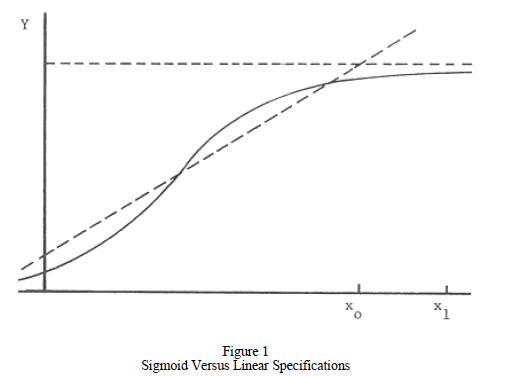
The mathematical problem appears immediately. A probability must satisfy:
whereas a linear predictor such as \(\beta_0+\beta_1X_{i1}+\cdots+\beta_kX_{ik}\) does not, in general, possess such bounds. It may produce numbers below zero or above one. A linear probability model can be useful in certain contexts as an approximation and has some interpretive advantages, but this incompatibility between the range of the linear predictor and the range of a probability constitutes a fundamental reason to seek another specification.
We do not need to abandon the linear predictor. What we can do is transform the probability.
2. From probability to odds and the logit
If \(0<P_i<1\), we can construct the ratio:
This quantity is commonly called the odds. It compares the probability that the event occurs with the probability that it does not.
For example, if \(P_i=0.75\):
The odds are therefore 3 to 1 in favor of the event. This transformation removes the upper bound of the probability, but it does not remove all restrictions:
Odds remain necessarily positive. To obtain a quantity capable of spanning the entire real line, we apply the natural logarithm:
This transformation is the logit of the probability:
We now have a quantity whose range is compatible with that of a linear predictor. We may therefore specify:
The probability \(P_i\) lies in the interval \((0,1)\); the odds \(P_i/(1-P_i)\) lie in \((0,\infty)\); and the log-odds, or logit, range across the entire real line \((-\infty,\infty)\). These are three different scales and should not be confused.
3. The logistic function
Once the preceding relation has been established, we can solve for \(P_i\). We begin from:
Applying the exponential function:
Through algebraic manipulation:
We have arrived at the standard logistic function. The transformation solves precisely the problem of interest: \(Z_i\) may take any real value, while the output of the function always lies between zero and one.
If \(Z_i\rightarrow-\infty\), then \(P_i\rightarrow0\).
If \(Z_i=0\), then \(P_i=0.5\).
If \(Z_i\rightarrow+\infty\), then \(P_i\rightarrow1\).
The function is continuous, smooth, and monotonically increasing. Its shape is the familiar sigmoid, or S-shaped curve. The standard logistic function also possesses rotational symmetry around the point \((0,1/2)\).
A more general expression of the logistic function is:
where \(L\) determines the upper limit, \(k\) regulates the rate of growth, and \(x_0\) determines the position of the midpoint. The standard logistic function commonly used to transform a linear predictor into a probability corresponds to:
It is also important to distinguish the logistic function used here as the inverse of the link function from the logistic distribution. The two objects are related, but they are not synonymous.
4. Why a logistic function?
Finding a mathematically convenient function does not, by itself, settle the problem of specification. As Aldrich and Nelson (1984) observe, many functions can transform an unrestricted predictor into a probability. The logistic function is not the only possibility.
Among the best-known alternatives is the probit model, which uses the standard normal cumulative distribution function as the inverse link. Another possibility is the complementary log-log link. Each choice imposes a different mathematical structure on the relationship between the predictor and the probability.
| Model | Link function | Main feature |
|---|---|---|
| Logit | \(\log[p/(1-p)]\) | Natural interpretation through odds and odds ratios. |
| Probit | \(\Phi^{-1}(p)\) | Uses the cumulative normal distribution. |
| Complementary log-log | \(\log[-\log(1-p)]\) | Introduces an asymmetric probability response. |
Logit and probit often produce very similar empirical results in a wide range of applications, particularly in the central regions of their respective curves. This does not mean that they are mathematically identical, nor that the choice between them can always be treated as irrelevant. The proper criterion remains substantive and statistical: what structure is justifiable for the phenomenon, what inferential properties are needed, and what aspects of the response one wishes to represent.
The availability of a statistical model does not constitute evidence that the model corresponds to the object. Choosing a link function is itself a hypothesis about the mathematical form of the relationship under study.
5. The statistical model
Up to this point we have examined mainly the geometry of the transformation. But logistic regression is not merely the drawing of an S-shaped curve. It is a probabilistic model.
When each observation represents an individual dichotomous outcome, the natural formulation is:
with:
If, by contrast, observations are grouped and we record \(Y_i\) successes out of \(n_i\) trials, we may write:
This distinction matters. It is not precise simply to say that “the data set follows a binomial distribution.” The probability distribution is specified for the response variable conditional on the covariates and depends on the observational structure of the data.
In the language of generalized linear models, logistic regression combines three elements:
Random component: a Bernoulli or binomial response.
Systematic component: the linear predictor \(X_i\beta\).
Link function: \(g(P_i)=\log[P_i/(1-P_i)]\).
The logistic function \(g^{-1}(Z)=1/(1+e^{-Z})\) is therefore the inverse of this link.
6. Estimation by maximum likelihood
The coefficients of a logistic regression are not usually obtained by minimizing the sum of squared residuals as in ordinary linear regression. They are estimated by maximum likelihood.
For conditionally independent Bernoulli observations, the contribution of each observation to the likelihood can be written as:
For \(n\) observations:
The procedure searches for the parameter values \(\beta\) that make the actually observed outcomes most likely under the specified model. In practice, one normally maximizes the logarithm of the likelihood:
In general there is no closed-form expression analogous to the ordinary least squares formula for obtaining the coefficients. The solution is found through iterative numerical procedures.
7. How to interpret the coefficients
This is one of the points that most often generates confusion when moving from linear to logistic regression. If:
then \(\beta_j\) does not directly represent the change in probability produced by a one-unit increase in \(X_j\). It represents the change in the log-odds, holding the other variables in the predictor constant.
Exponentiating the coefficient gives a more intuitive interpretation:
This is the factor by which the odds are multiplied when \(X_j\) increases by one unit, ceteris paribus.
If \(\beta_j=0.5\), then:
A one-unit increase in \(X_j\) multiplies the odds by approximately 1.65, that is, increases them by approximately 65%, holding the other variables constant. This does not mean that the probability rises by 0.5 or by 50 percentage points.
The effect on probability is not constant
The reason is that the relationship between \(Z_i=X_i\beta\) and \(P_i\) is nonlinear. For a continuous variable \(X_j\), under the simple additive specification, the marginal effect is:
Thus, the same coefficient \(\beta_j\) may correspond to different changes in probability depending on the point of the curve at which each observation lies. The response is more sensitive in the central region of the logistic function and less sensitive near its extremes.
This is not an accidental difficulty of the model. It is a direct consequence of the mathematical structure we have chosen to use.
8. Evaluation and diagnostics
Estimating a set of coefficients does not settle the problem. We must ask whether the model adequately describes the information we seek to explain and, above all, whether the inferences we wish to draw from it are defensible.
Likelihood-ratio test
A classical comparison contrasts a model containing explanatory variables with a model containing only the intercept. The likelihood-ratio statistic can be written as:
and, under regularity conditions, it approximately follows a chi-squared distribution with degrees of freedom corresponding to the number of restrictions being tested.
This test can indicate whether the set of predictors improves fit relative to a more restricted model. It should not, however, be confused with a complete evaluation of the model’s scientific usefulness.
Statistical significance is not enough
Depending on the purpose of the investigation, one should also examine aspects such as:
- the calibration of estimated probabilities;
- the ability to discriminate between outcomes;
- deviance and residuals appropriate to generalized linear models;
- the stability of the coefficients;
- the presence of influential observations;
- out-of-sample performance when the objective is predictive;
- and, above all, the adequacy of the functional form and assumptions to the scientific problem.
9. Specification returns to the center
We thus return to the problem with which we began. Logistic regression elegantly solves a mathematical difficulty: it allows an unrestricted predictor to be related to a probability necessarily bounded between zero and one. But this mathematical virtue does not make the logit an automatic choice for every dichotomous phenomenon.
Its use presupposes a particular structure. Among other things, one should examine whether the linear predictor is an adequate representation of the log-odds, whether dependence among observations has been modeled correctly, whether relevant interactions or nonlinearities are present, and whether complete or quasi-complete separation occurs, a circumstance capable of producing problematic or non-finite maximum-likelihood estimates.
- Is there a scientific justification for the variables included and for the way in which they enter the predictor?
- Does the approximately linear relationship assumed actually hold for the log-odds, or are transformations, nonlinear terms, or interactions required?
- Is the dependence structure among observations represented adequately?
- Is there enough information in the data to identify the parameters?
- Is the purpose explanatory, predictive, descriptive, or causal?
The last question deserves particular attention. An association obtained through logistic regression does not become causal merely because it has been expressed through coefficients, probabilities, or odds ratios. Causality requires assumptions and a design capable of justifying such an interpretation.
Likewise, a model may be a useful approximation without being a literally exact description of the data-generating process. The scientific problem is then to determine which properties of that approximation are sufficiently robust for the specific inferential purpose.
The broader lesson therefore extends beyond logistic regression. A statistical model is a mathematical instrument containing a specific structure: a space of possible outcomes, a probability distribution, a functional form, parameters, and assumptions concerning the relationships among magnitudes. To apply it is to affirm—explicitly or implicitly—that these properties bear some relevant correspondence to the phenomenon under study.
From this standpoint, the problem of specification has a genuinely epistemological content. Mathematics is not a decoration subsequently placed upon the data. Nor do the data, by themselves, determine which model must be used. Between the real object and the mathematical expression there is a theoretical mediation that must be examined, criticized, and tested.
The logit constitutes a particularly elegant solution because it transforms a restricted probability into an unrestricted quantity and subsequently allows a valid probability to be recovered through the logistic function:
But the elegance of the transformation does not replace the investigation of the object. Precisely because the model possesses determinate mathematical properties, we must ask when those properties are pertinent. There lies the point of contact between statistics, mathematics, and scientific knowledge.
References
Aldrich, J. H., & Nelson, F. D. (1984). Linear Probability, Logit, and Probit Models. Beverly Hills: Sage University Papers Series, Quantitative Applications in the Social Sciences.
Liao, T. F. (1994). Interpreting Probability Models: Logit, Probit, and Other Generalized Linear Models. Sage University Papers Series, Quantitative Applications in the Social Sciences.
McCullagh, P., & Nelder, J. A. (1989). Generalized Linear Models (2nd ed.). London: Chapman & Hall.
Leave a Comment/Deja un Comentario