
Political Economy · Quantitative Methods
Measuring Sectoral Interrelationships in the U.S. Economy
An empirical methodology using make and use tables, 1997–2019
Social production connects activities that, considered in isolation, appear independent. An industry transforms commodities produced by others; its own products, in turn, enter new production processes. Studying these connections requires linking the analysis of economic structure to instruments that make its relationships observable.
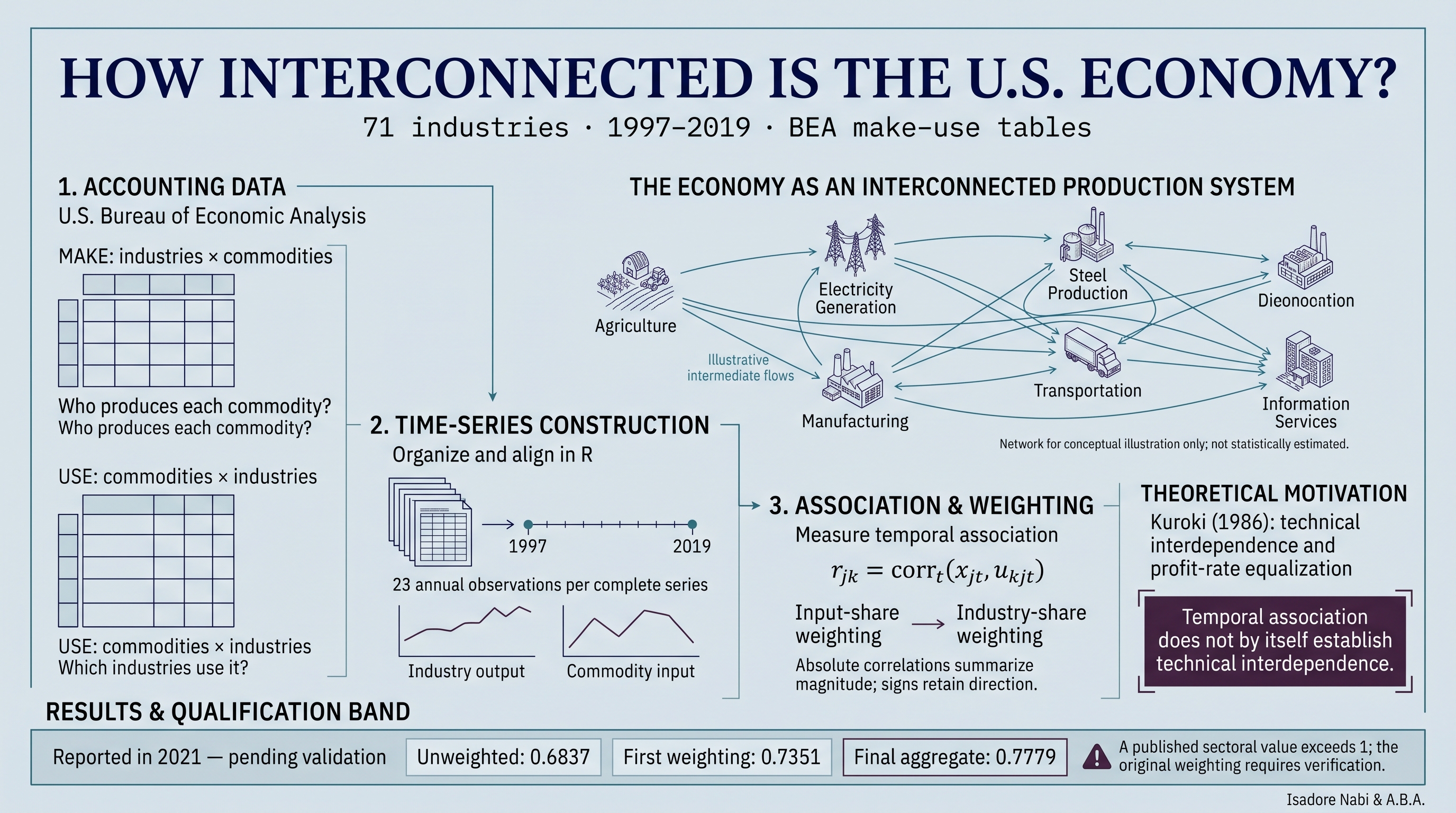
This article presents a strategy for organizing annual make and use tables into comparable time series and constructing a descriptive indicator of the association between output and inputs. The original study used BEA data for 71 U.S. industries between 1997 and 2019, processing in R, and two levels of weighting applied to absolute correlations. This edition makes the notation explicit, distinguishes commodities from industries, and preserves the published figures as historical results subject to verification.
per complete series
01 / MotivationThe economic problem
From the standpoint of Marxist political economy, the study of branches of production acquires meaning within the reproduction of society as a whole. The division of labor multiplies specializations, but also the material connections required to sustain each activity.
The question guiding this research is how to develop an empirical approximation to the interconnectedness of production using disaggregated accounting data. Input-output accounts provide a particularly useful basis: they allow us to examine what is produced, what is used as an input, and how the uses of commodities are distributed.
The central theoretical antecedent is Kuroki’s discussion of the equalization of the rate of profit and technical interdependence in the volume edited by Semmler. The reference is to the 1986 publication of the proceedings of a conference held in 1985.[1] Connecting this discussion to an empirical indicator requires explaining which relationship is observed and how it relates to the model’s categories.
The empirical task is to make explicit the link between an economic category and the statistical operation used to study it.
It is therefore useful to distinguish three dimensions: the existence of production flows, their relative importance, and the temporal association between their magnitudes. These dimensions complement one another, but each answers a different question.
02 / Statistical foundationData and units of analysis
Reading the files correctly requires identifying the accounting framework. The BEA distinguishes the make and use tables of the make–use framework from the tables of the supply–use framework. In particular, a supply table includes imports and should not automatically be treated as synonymous with domestic production.[2]
| Object | Rows | Columns | Contents |
|---|---|---|---|
| Make table, V | Industries j | Commodities k | Output of each commodity by each industry. |
| Intermediate use table, U | Commodities k | Industries j | Inputs of each commodity used by each industry. |
| Industry output, x | One observation per industry | Vector | Total output of all commodities produced by an industry. |
Source: the structure described in the BEA’s input-output accounts manual. Check the orientation of each exported table before using its totals.
Let vjkt denote the output of commodity k produced by industry j in year t, and let ukjt denote that industry’s intermediate use of commodity k. With this orientation, industry output is obtained by summing the industry’s row across the commodity block:
The bottom totals row of a make table with this orientation reports commodity totals, whereas industry totals are obtained by summing across rows. Selecting a spreadsheet position without checking its meaning can change the variable being analyzed.[3]
The original screenshots identify tables after redefinitions and uses valued at producers’ prices. A replication must maintain consistent valuation, classification, and treatment of redefinitions across both tables and over time. Updates to a statistical database can revise its historical figures.
03 / PreparationFrom annual tables to time series
Data preparation consists of aligning identifiers and observations. A single year provides a cross section; successive years make it possible to construct a dataset with both industry and time dimensions. Each industry then has an output series and a series for each input category.
- Select compatible tables.
Identify the data vintage, monetary units, aggregation level, and treatment of redefinitions. Separate the production blocks from rows and columns containing totals, value added, and final demand.
- Obtain output by industry.
Construct each year’s vector x from verified industry totals. Retain codes as identifiers; names serve as descriptions.
- Reorient the use block where useful.
Transposing U places industries in rows and commodities in columns. This facilitates combining records while preserving the meaning of each flow: it changes its position, not its economic nature.
- Stack the years and align the keys.
Construct a table with one row per industry–year combination. Check that each combination appears only once and that inputs retain a consistent classification.
- Construct comparable series.
For each industry, assemble output and each input over the same years. Record missing values, zeros, classification changes, and constant series before calculating correlations.
- Calculate, weight, and retain the outputs.
Save signed coefficients, their absolute values, the observations used, the weights, and the aggregate indicators. Validation must make each result traceable to its input data.
| Year | Industry | Output | Input 1 | Input 2 | … |
|---|---|---|---|---|---|
| 1997 | j | xj,1997 | u1j,1997 | u2j,1997 | … |
| 1998 | j | xj,1998 | u1j,1998 | u2j,1998 | … |
| ⋮ | ⋮ | ⋮ | ⋮ | ⋮ | ⋱ |
| 2019 | j | xj,2019 | u1j,2019 | u2j,2019 | … |
A complete series has 23 observations. A balanced dataset with 71 industries and one row per industry–year contains 1,633 rows; the number of columns depends on the selected input block.
04 / MeasurementTemporal output–input association
For each pair consisting of an industry and a commodity used as an input, Pearson’s correlation is calculated between the two series. The time index runs through the comparable years; this is not a correlation across industries within a single year.
The sign distinguishes movements in the same direction from movements in opposite directions. To summarize their intensity alone, we use ajk = |rjk|. Both matrices should be retained: a large negative coefficient contains economic information that disappears when its absolute value is taken.
Pearson’s correlation is undefined for a constant series. A flow that is zero in every year should likewise not automatically be assigned a correlation of zero. When data are missing, the number of observations underlying each coefficient must be reported, and an explicit comparison rule must be maintained.
05 / AggregationThe two levels of weighting
Weighting incorporates the economic importance of flows. The first level summarizes each industry’s association with its inputs; the second aggregates the industry results.
First level: input composition
Because each correlation summarizes several years, the weights must represent an explicitly defined temporal distribution. One can select a reference year, average annual shares, or calculate shares from cumulative flows. These choices can produce different results.
One possible convention for a new replication is to use shares based on cumulative flows over the period:
When a correlation is undefined and its input has a positive weight, the series must be reviewed, or its exclusion and the renormalization of the remaining weights must be made explicit. Removing missing values without adjusting the denominator changes the indicator.
Second level: industry shares
For example, qj could be defined as the industry’s share of cumulative gross output across all included industries. This choice must also be documented and distinguished from weighting by value added.
The equations above specify a family of indicators. Their exact application depends on the selected weights and data coverage. With normalized nonnegative weights, the sectoral and overall indicators necessarily lie within the interval [0, 1].
06 / Worked exampleInterpreting the weighting
Consider an industry with two input categories. The first has a correlation of 0.90 with output and accounts for 80% of its inputs; the second has a correlation of −0.20 and accounts for the remaining 20%.
The simple mean of the two magnitudes would be 0.55. The weighted result is higher because the stronger association corresponds to the input with the larger share. Weighting expresses an economic choice; an increase in the indicator does not, by itself, improve the evidence.
If another industry scores 0.40 and the industry shares are 0.60 and 0.40, respectively, the overall indicator is:
07 / Published evidenceResults and verification note
The R outputs reproduced in the original publication show the following figures. They are transcribed to preserve documentary traceability; this edition neither recalculates the dataset nor certifies that the results have been reproduced.
| Stage | Reported value | Documentary interpretation |
|---|---|---|
| Mean of absolute correlations | 0.6837338 | Summary before economic weighting. |
| Mean of industry indicators | 0.7351034 | Output associated with the first level of weighting. |
| Aggregate with industry weighting | 0.7778624 | Final reported output. |
Sources: the first output, second output, and final output from the original publication.
Correlation r must also be distinguished from the coefficient of determination R2. An average of absolute correlations cannot be presented as a proportion of explained variance. The familiar relationship R2 = r2 applies to simple linear regression with an intercept, not to this aggregation of multiple pairs.[4]
Finally, describing a correlation as “strong” requires a contextual criterion. If 0.70 is chosen as a descriptive reference, its distance from 0.6837338 is 0.0162662 indicator units. Proximity to that threshold neither replaces validation of the calculation nor establishes an economic conclusion.
08 / DiscussionInterpretation and scope
What this strategy can investigate
Once the data and calculations have been validated, the procedure allows comparisons of industry profiles of temporal association and an examination of how their synthesis changes when economic weights are introduced. Its usefulness also lies in making the passage from accounting tables to time series and indicators traceable.
Checks that would strengthen inference
- Prices and trends. Examine how much of the association between monetary magnitudes reflects price changes or common trends. Depending on the question, compare levels, deflated series, growth rates, or justified time-series specifications.
- Temporal dependence and stability. Examine autocorrelation, influential observations, and possible breaks. Statistical tests must respect the temporal structure of the data.
- Aggregation decisions. Compare weights and coverage, retain sign information, and document the treatment of commodities associated with the industry’s own sector.
- Structural content. Compare the indicator with measures based on flows and production requirements. Temporal comovement and the technical intensity of a linkage are distinct dimensions.
These checks are proposed extensions. They are not presented as tests already performed in the 2021 study.
Correlations between trending series can invite misleading interpretations; time-series techniques help distinguish these movements from more stable relationships.[4] Gross output also incorporates intermediate inputs within an accounting identity. This connection must form part of the economic interpretation of the result.
The connection to Marxist debate
Empirical research can contribute to debates on reproduction, competition, and the interconnectedness of branches of production. Connecting this indicator to the dynamics of the rate of profit requires justifying the step from observed association to the technical interdependence relevant to the model.
The United States provides a relevant setting for investigation. Its analysis alone neither establishes a universal regularity nor verifies every condition of a theoretical result on stability. Comparisons across periods, countries, and structural measures would allow the generality of the hypothesis to be assessed.
A study becomes stronger when its data, its operations, and the scope of its conclusions can be examined separately.
The contribution worth developing is a reproducible strategy for organizing production data and examining a hypothesis about economic interconnectedness. Reviewing the published calculation and conducting robustness checks are the next steps toward consolidating that contribution.
09 / MaterialsReplication and traceability
The materials archive linked at the end corresponds to the resource provided by the authors in the original post. A complete replication should retain both the downloaded files and the transformations produced by the code.
- Record the source: download date, data vintage, tables, units, valuation, and industry and commodity codes.
- Verify alignment: unique keys, annual coverage, classification changes, and correspondence between output and uses.
- Audit the coefficients: variation in the series, number of observations, missing values, and the range of each correlation.
- Audit the weights: temporal definition, positive denominators, nonnegative weights, and a sum of one at each level.
- Publish the outputs: signed and absolute-value matrices, weights, sectoral results, and the overall aggregate, together with the versions of R and its packages.
Range checks are especially useful: an indicator of the form described must remain between zero and one. If an output violates that property, interpretation should pause while the operation generating it is located.
10 / SourcesReferences and further reading
- [1] Kuroki, R. (1986). The equalization of the rate of profit reconsidered. In W. Semmler (Ed.), Competition, instability, and nonlinear cycles (pp. 35–50). Springer. Publisher’s record. Conference held in March 1985; publication year corrected according to the publisher.
- [2] U.S. Bureau of Economic Analysis. (n.d.). Guide to the interactive industry input-output accounts tables. Read the guide.
- [3] U.S. Bureau of Economic Analysis. (2006). Concepts and methods of the U.S. input-output accounts. Methodological manual.
- [4] Hyndman, R. J., & Athanasopoulos, G. (2021). Forecasting: Principles and practice (3rd ed.). OTexts. Chapter 7: Time series regression models. Read the chapter.
- [5] U.S. Bureau of Economic Analysis. (n.d.). Input-output. Access to tables and code concordances. Explore the data.
Debate bibliography and sources listed in the original publication
Retained as a bibliographic guide to the 2021 article; the works listed are not presented as an exhaustive review of the current state of research. Non-English publication titles are retained in their original language.
- Cockshott, P., & Cottrell, A. (2005). Robust correlations between prices and labor values. Cambridge Journal of Economics, 309–316.
- Cockshott, P., Cottrell, A., & Valle Baeza, A. (2014). The empirics of the labour theory of value: Reply to Nitzan and Bichler. Investigación Económica, 115–134.
- Cockshott, P., Cottrell, A., & Zachariah, D. (2019). Against the Kliman theory. Document linked in the original.
- Kliman, A. (2002). The law of value and laws of statistics: Sectoral values and prices in the US economy, 1977–97. Cambridge Journal of Economics, 299–311.
- Kliman, A. (2005). Reply to Cockshott and Cottrell. Cambridge Journal of Economics, 317–323.
- Kliman, A. (2014). What is spurious correlation? A reply to Díaz and Osuna. Journal of Post Keynesian Economics, 345–356.
- Mindrila, D., & Balentyne, P. (n.d.). Scatterplots and correlation. University of West Georgia. Notes linked in the original.
- Nabi, I. (2021). Sobre la metodología del U.S. Bureau of Economic Analysis para la redefinición y reasignación de productos en la matriz insumo-producto de Estados Unidos. Related post.
- Sánchez, C., & Ferràndez, M. N. (2010). Valores, precios de producción y precios de mercado a partir de los datos de la economía española. Investigación Económica, 87–118.
- Sánchez, C., & Montibeler, E. E. (2015). La teoría del valor trabajo y los precios en China. Economia e Sociedade, 329–354.
- U.S. Bureau of Economic Analysis. (2021). The make of commodities by industries, after redefinitions; The use of commodities by industries, after redefinitions (producers’ prices). Tables used in the original study.
- Zachariah, D. (2006). Labour value and equalisation of profit rates: A multi-country study. Indian Development Review, 4, 1–20.
Leave a Comment/Deja un Comentario