
On Principal Component Analysis (PCA)
Geometric intuition, algebraic foundations, statistical interpretation, and the epistemological scope of dimensionality reduction
Representing a phenomenon through many variables allows a rich description, but can also make its principal relationships harder to identify. Principal component analysis—PCA—constructs new coordinates to study the joint variation of those variables. The decisive question is how to reduce a representation’s complexity without losing sight of what is preserved, what is discarded, and under which conditions its interpretation is legitimate.
This essay develops PCA through four connected perspectives: a geometric transformation of a cloud of observations; a constrained optimization problem; a matrix decomposition; and a tool for scientific exploration and interpretation. It retains the gene-expression and financial-assessment examples, component-retention criteria, graphical diagnostics, Mahalanobis distance, the discussion of NIPALS, and the comparison with linear regression. Mathematical derivation, reproducibility, and the conditions supporting inference are expanded.
Editorial note. All thematic strands and 51 figures from the 2021 document are preserved. Formulations requiring greater precision are revised in the main discussion; the original images are collected without cropping in the visual archive and retain their attributions. The historical Spanish PDF remains available at the end.
I. Variables, attributes, and dimensionality
A dataset organizes observations of particular units of study: people, animals, firms, territories, products, or states of a physical system. Each unit is described by variables. When p numerical variables are recorded for n units, the usual representation is a matrix X of size n × p: rows correspond to observations and columns to variables. Each row can be interpreted as a point in the feature space ℝp.
The word attribute requires clarification. In data science it may designate a measured feature; in R it also refers to metadata associated with an object, such as its dimensions, names, or class. Adler’s observation about the importance of attributes in R objects is relevant to understanding their computational representation, but such metadata should not automatically be identified with the statistical variables in an investigation. A class attribute can change how R interprets an object without adding a dimension to the measured phenomenon. [1]
The dimensionality of a representation is the number of coordinates used. Intrinsic dimensionality, by contrast, refers to the degrees of freedom needed to describe the underlying structure under the model being considered. A cloud lying approximately on a plane may have many coordinates while still admitting an approximately two-dimensional representation. With noise, effective dimensionality also depends on the approximation tolerance. There is not always a single minimum number independent of the purpose of the analysis.
Variable selection and component extraction
Dimensionality reduction encompasses different strategies. Variable selection retains a subset of the original columns; feature extraction constructs new variables from them. PCA belongs to the second family: a component may combine information from all the initial variables. By definition, it does not identify which columns should be removed or solve a combinatorial search over subsets. Such problems can be connected to PCA, but they have different formulations.
This distinction also limits the meaning of “essential information.” In ordinary PCA, the operational criterion is the variance represented by a linear subspace. Whether that variation is essential to a biological, economic, or social explanation requires an additional argument about measurement, scale, context, and the research question.
II. Bellman, Pearson, and the problem of representation
The expression curse of dimensionality, associated with Richard Bellman, brings together difficulties that arise as the number of dimensions increases: growing computational costs for certain procedures, relative sparsity of observations, reduced effectiveness of some notions of neighborhood, and the need to impose structure on the problem. On a grid with ten positions per axis, systematically exploring p dimensions produces 10p combinations. This illustrates exponential growth; it is not a universal law requiring every statistical method to use exactly that amount of data. [3]
The difficulty depends on the problem, distribution, regularity, and relationships among variables. It is therefore useful to distinguish feature space from the sample space of probability theory: the former organizes observable coordinates, whereas the latter contains the possible outcomes of an experiment. They can be connected through random variables, but the concepts are not interchangeable.
In 1901, Karl Pearson studied lines and planes of closest fit to systems of points. His geometric approach approximates a cloud by a line or plane by minimizing the sum of squared orthogonal distances. Hotelling’s later formulation helped establish principal component analysis as a multivariate technique. This genealogy predates the contemporary vocabulary of machine learning. [11] [22]
The original document politically characterizes Pearson as a Marxist. The question of the relationship between intellectual biography, the history of statistics, and philosophy of science is retained here, but that classification requires a dedicated historical investigation and is not used as a premise in deriving PCA. The method’s mathematical validity and the historical assessment of its author belong to different levels of argument that must be supported separately.
Pearson’s line provides a useful intuition: an elongated cloud can be described relatively accurately by a coordinate along its dominant direction. Identifying that direction, however, does not establish a cause of the phenomenon. The fit describes a structure of variation in the measurements; explaining it requires additional theory and evidence.
III. Definition and optimization of PCA
Let x be a random vector of p variables, μ its mean, and Σ its covariance matrix, assuming finite second moments. The first principal component is a linear combination of the centered variables with maximum variance, subject to a normalization constraint on its coefficients. In sample analysis, the population covariance is replaced by its estimate S.
maximize aTΣa, subject to aTa = 1.
The vector a₁ defines a direction; the component is the variable obtained by projecting onto it. The unit-length constraint prevents artificially increasing variance by multiplying all coefficients by a constant.
Without this constraint, multiplying a by an arbitrarily large number would increase the combination’s variance without bound. Normalization makes variation along different directions comparable. The second component maximizes the remaining variance, with a unit coefficient vector orthogonal to the first. The procedure continues successively.
subject to aTa = 1 and aTaℓ = 0 for ℓ < k.
Each new direction is chosen in the orthogonal complement of the preceding ones. This formulation characterizes the solution independently of the algorithm used to compute it.
The Lagrangian for the first direction is L(a, λ) = aTΣa − λ(aTa − 1). The stationarity condition leads to Σa = λa. The principal directions are therefore eigenvectors of the covariance matrix, and their variances are the corresponding eigenvalues. The first direction is associated with the largest eigenvalue; the remaining directions are ordered in decreasing order. If eigenvalues are repeated, a particular basis for the associated subspace may not be unique.
The mathematical interpretation has two levels. Eigenvectors specify how to combine the original coordinates; eigenvalues quantify variation along those combinations. Observation scores show where each unit of study lies in the new coordinate system. Keeping these three objects separate avoids confusing weights, observations, and amounts of variation.
The direction tells us how to look at the data; the score locates an observation in that view; the eigenvalue measures how much variation appears along it.
IV. Two genes and six mice
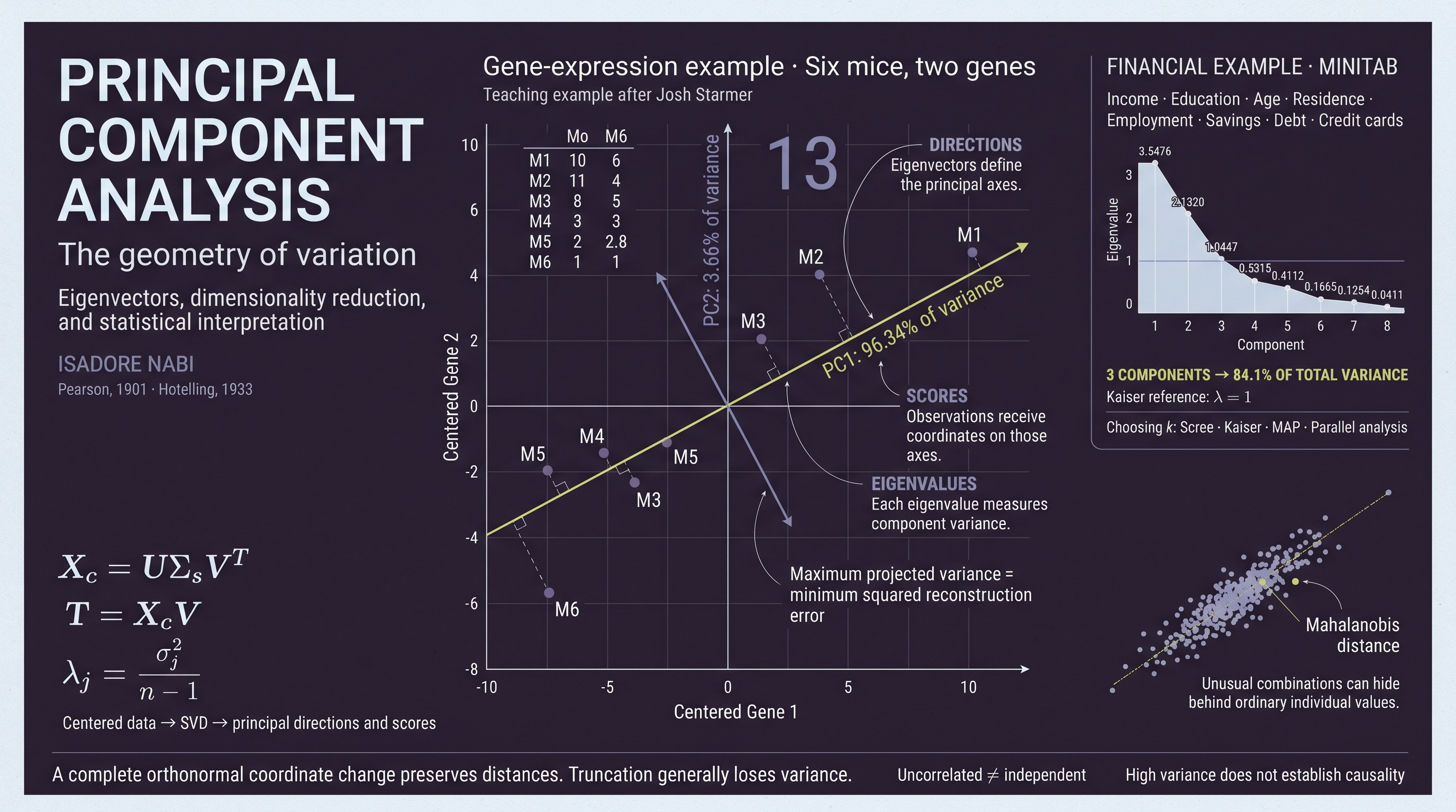
Following Josh Starmer’s teaching example used in the original document, consider six mice described by expression measurements for two genes. The mice are the units of study and the genes are the variables. Transcription is the synthesis of RNA from DNA; it must be distinguished from translation, which produces proteins. The quantities are retained as teaching values: no experimental unit or biological precision undocumented by the example is attributed to them. [13]
| Mouse | Gene 1 | Gene 2 |
|---|---|---|
| 1 | 10 | 6 |
| 2 | 11 | 4 |
| 3 | 8 | 5 |
| 4 | 3 | 3 |
| 5 | 2 | 2.8 |
| 6 | 1 | 1 |
In a two-dimensional plot, each mouse occupies the position defined by its two measurements. The first three have relatively high values for both genes, while the remaining mice have lower values. The cloud allows us to ask questions about covariation and grouping, but a figure alone does not establish population differences or causal mechanisms.
The first step in centered PCA is to subtract each variable’s mean. For these values, the mean of gene 1 is approximately 5.8333 and that of gene 2 is 3.6333. The centroid moves to the origin; differences between pairs of observations remain unchanged.
Xc = X − 1x̄T.
The superscript c denotes centering; 1 is a column vector of n ones. Centering is not the same as dividing by standard deviations.
Starmer’s original sequence is preserved in full in the visual archive. The new figure shows the same six centered points, with the principal direction computed from the table and the orthogonal residuals involved in the fitting criterion.

The example teaches the geometric mechanics. An actual gene-expression study requires attention to measurement, sequencing depth, appropriate transformations, batch effects, replication, and uncertainty. PCA on an unprepared count table may reflect technical magnitudes before biological differences of interest.
V. Transformations, structure, and preservation
A transformation is a mapping between spaces. It may be linear, affine, or of another kind. It need not map a domain into the same set: in general, we write f: D → C, and its image is the set of values actually reached in the codomain. For ordinary PCA, translations, orthogonal coordinate changes, and projections onto subspaces are especially important.
| Transformation | Characterization | Important distinction |
|---|---|---|
| Translation | x ↦ x + b | Preserves distances and differences between points; generally not linear because it does not fix the origin. |
| Rotation | x ↦ Qx, with QTQ = I and det Q = 1 | Preserves inner products, norms, angles, and distances. |
| Reflection | An orthogonal transformation reversing orientation | Also preserves distances. An orthogonal matrix may combine rotations and reflections. |
| Uniform dilation or contraction | x ↦ cx | Multiplies all distances by |c|; an isometry only when |c| = 1. |
| Stretching along one or more axes | x ↦ Dx, with D diagonal | Changes relative geometry when scale factors differ. |
| Shear | A linear deformation that shifts coordinates according to other coordinates | May preserve area or volume in particular cases, but generally alters angles and lengths. |
| Orthogonal projection | x ↦ Px, with PT = P and P² = P | Generally not invertible; dimensionality reduction may contract distances and map distinct points onto the same point. |
Isomorphism, homeomorphism, and isometry
An isomorphism preserves the specified structure: for example, addition and scalar multiplication in vector spaces. A homeomorphism is a continuous bijection with a continuous inverse. An isometry preserves distances; when also surjective, it establishes an equivalence between metric spaces. These notions are related, but none should be used indiscriminately in place of the others.
Preserving topology does not imply preserving a norm or metric: multiplying all coordinates by two provides an elementary counterexample. The transformation is a homeomorphism of ℝp and changes every nonzero distance. Similarly, a translation preserves distances without being a linear isomorphism under the original vector operations, unless it is the zero translation.
In an inner-product space, the Euclidean norm is defined by ‖x‖ = √⟨x,x⟩ and the induced distance by d(x,y) = ‖x − y‖. The norm measures vector length; the metric measures distance between points. Hilbert spaces generalize this framework to complete inner-product spaces. These extensions situate PCA within a broader mathematical landscape, but they do not justify transferring its properties to any normed space without proof.
The philosophical discussion of matter and form
The original reflection on Aristotle and Plato can be retained as a question about the connection between a system’s elements and the relations organizing them. This philosophical interpretation should nevertheless be distinguished from the mathematical definition of structure. Classifying objects “up to isomorphism” means grouping them according to a specified structural equivalence; it does not mean that they belong to any classification whatsoever or to none at all.
From a materialist perspective, mathematical abstraction can be examined as an operation that selects properties of concrete phenomena to study particular relations. The critical requirement is to state what is abstracted and what is preserved. In PCA, certain properties are preserved exactly under a complete orthonormal change of basis; others are only approximated when coordinates are discarded. Philosophical analysis becomes more precise when it starts from that distinction.
VI. Orthogonal projection and reconstruction
Let a be a unit vector defining a line through the origin, and let z be a centered observation written as a column vector. Its coordinate along that line is t = aTz. Its projection in the original space is ẑ = aaTz. The difference e = z − ẑ is perpendicular to the projection direction.
‖z‖² = ‖ẑ‖² + ‖e‖².
The Pythagorean theorem decomposes squared length into a represented part and a residual part.
For a fixed centered cloud, the sum of ‖z‖² over all observations is constant. Maximizing the sum of squared projected lengths therefore equals minimizing the sum of squared orthogonal residuals. This equivalence requires the same geometry, the same dataset, and comparison of subspaces of equal dimension.
The two formulations do not distinguish an “analytical” PCA from a “numerical” one. They are mathematically equivalent objectives that can be solved using different algorithms.
Squaring is essential. Minimizing a sum of unsquared distances generally defines a different problem and may lead to another solution. Nor must components be computed through the Minkowski or Cauchy–Schwarz inequalities: these tools help prove properties of norms and inner products, but do not replace a specification of the optimization procedure.
A projection is a linear transformation that can be defined without choosing coordinates. Once a basis is chosen, it has a precise matrix representation; there is no opposition between a “purely mathematical” projection and a “merely computational” matrix. For a subspace whose orthonormal columns are collected in Vk, the projection matrix is Pk = VkVkT.
The original discussion of projective geometry is retained as context, with a qualification: the orthogonal projection of PCA belongs here to Euclidean geometry and linear algebra. It need not be conflated with the whole of projective geometry, whose historical development was collective and cannot simply be attributed to Lobachevsky.
In several dimensions, the criterion is written as minimization of the Frobenius norm of the reconstruction residuals. Approximation by the first k components is optimal among approximations of rank at most k under this quadratic loss. “Optimal” always means optimal for a declared criterion, not for every possible scientific purpose.
‖Xc − X̂c,k‖F² = (n − 1) ∑j>k λj.
This identity uses eigenvalues of the sample covariance with divisor n − 1. To reconstruct the original coordinates, add the mean; if variables were standardized, also reverse the scaling.
VII. Slope, unit vectors, and components
The original geometric explanation uses a line with slope 0.25, represented by a displacement of four units along the first axis and one along the second. Its direction vector is (4,1)T. Its length is √17 ≈ 4.1231; dividing its coordinates by that length yields a unit direction.
a2 = (−1,4)T/√17 ≈ (−0.2425, 0.9701)T.
The vectors have unit norm and zero inner product. The rounded values 0.97 and 0.242 in the original material illustrate this normalization.
The line can be written as y = 0.25x; its slope equals the derivative of this linear function. But the coefficients of a principal direction are not generally “derivatives of the phenomenon.” Here, slope is the ratio of the direction vector’s coordinates. The unit eigenvector contains a normalized representation of that direction and is determined by the covariance structure of the data.
Normalizing (4,1) does not standardize each observation or transform the data into a normal distribution. Nor does it make a cloud’s mean zero. It produces a unit-length vector. With that direction, an observation’s first centered coordinate would be approximately t1 = 0.9701x1c + 0.2425x2c; the second would be t2 = −0.2425x1c + 0.9701x2c.
The direction (4,1) belongs to the original graphical explanation. Axes computed exactly from the six-mouse table may differ from that teaching slope. For traceability, the new figure and numerical table in this edition use the SVD of the transcribed values, while the visual archive preserves the original construction.
The Cauchy–Schwarz inequality guarantees that |⟨x,a⟩| ≤ ‖x‖‖a‖ and helps bound the length of a projection. The Minkowski inequality expresses the triangle inequality for Lp norms, with p ≥ 1. Pythagoras provides an exact identity when components are orthogonal in an inner-product space. These relationships serve different purposes; they are not three alternative algorithms for “finding” components.
VIII. Eigenvalues, eigenvectors, and SVD
For the centered matrix Xc, with observations in rows, sample covariance is S = XcTXc/(n − 1). This matrix is real, symmetric, and positive semidefinite. By the spectral theorem, it admits an orthonormal basis of eigenvectors collected as columns of V. Its eigenvalues are real and nonnegative.
Λ = diag(λ1, …, λp), λ1 ≥ ⋯ ≥ λp ≥ 0
T = XcV, Cov(T) = Λ.
V describes the directions and T contains the scores. The diagonal matrix Λ contains the variances and expresses sample uncorrelatedness between different components.
The singular value decomposition of the data matrix provides the same centered PCA solution. In reduced form, if the rank is r, we write Xc = UΣsVrT, with U of size n × r, Vr of size p × r, and diagonal Σs of size r × r. The subscript distinguishes singular values from population covariance.
λj = σj²/(n − 1), σj = √((n − 1)λj).
The singular values of Xc are square roots of the eigenvalues of XcᵀXc. To obtain component variances, the divisor n − 1 must be included.
What distinguishes the two decompositions
An SVD exists for any real rectangular or square matrix. Diagonalization by similarity requires a square matrix and is not always possible; for general matrices, eigenvalues may be complex and an eigenvector basis need not be orthogonal. These general qualifications, however, do not describe a difficulty of the covariance matrix in PCA: symmetry guarantees orthogonal diagonalization, and positive semidefiniteness guarantees nonnegative eigenvalues.
In a general diagonalization A = PDP−1, the outer matrices are inverses. In an SVD A = UΣVT, the matrices U and V have different roles and are not generally each other’s inverses. If rectangular, they do not even admit a two-sided inverse. In their complete square versions they represent orthogonal transformations; a reduced SVD contains orthonormal bases for subspaces.
The connection between eigenvectors and singular vectors is particularly direct in PCA, because the right singular vectors of Xc are eigenvectors of S. These are not two incompatible theories, but connected formulations for computing the same representation under the same centering and scaling conventions. [2] [4]
Explained variance and discarded variance
Ck = ∑j=1k ρj, Rk = 1 − Ck.
ρj is the proportion explained by component j; Ck is the cumulative proportion in the first k; Rk is the fraction of variance excluded from that representation. Positive total variance is assumed.
The eigenvalue of a retained component represents variation preserved along that axis, not “lost information.” Reconstruction loss is related to the sum of discarded eigenvalues. This quadratic relationship does not turn variance into a universal measure of meaning, causality, or information in Shannon’s sense.
IX. Centering, standardization, and matrix choice
Centering subtracts the mean. Standardization by z-scores subtracts the mean and divides by each variable’s standard deviation. Vector normalization, in the sense used above, divides by a norm. These are different operations, although all may informally be described as changes of scale.
R = ZTZ/(n − 1).
If sj is computed using divisor n − 1, the sample covariance of Z is the original variables’ correlation matrix R. Constant columns require prior treatment.
The z transformation produces mean zero and unit variance under the convention used. It does not impose normality: a skewed distribution remains skewed after an affine transformation with positive scale. Descriptive PCA can be computed without assuming multivariate normality; certain tests, intervals, or control limits do require additional assumptions.
| Basis of analysis | Interpretation | Substantive decision |
|---|---|---|
| Covariances | Centered variables are analyzed in their measurement scales. | May be appropriate when units are comparable and variance differences are meaningful. |
| Correlations | The covariance of standardized variables is analyzed. | Gives each variable the same initial variance; often relevant with heterogeneous units, although it may also amplify unreliable variables. |
A variable measured in thousands may dominate one measured in fractions if changing units increases its variance. But the magnitude of a variable’s mean does not, by itself, determine its variance. A scaling decision requires examination of dispersion, units, and purpose, rather than merely large or small absolute values.
Standardization changes the geometric problem by weighting the original coordinates differently. It should not be presented as a neutral operation that always improves analysis. It also matters whether standard deviation uses n or n − 1. In the same sample, consistently applying either divisor to all variables introduces only a common factor between the two standardizations; directions and explained-variance proportions coincide, but score magnitudes and variances change.
The connection to the same author’s essay on rescaling remains relevant. The web edition retains that link and emphasizes these distinctions so that both texts support each other without reproducing the confusion between standardization and transformation to a normal distribution. [9]
X. Orthogonality, uncorrelatedness, and rank
Two nonzero vectors with zero inner product are orthogonal and therefore linearly independent. The converse is false: two vectors may be linearly independent without being perpendicular. “Orthogonal” and “perpendicular” do not designate properties reserved for three and two dimensions respectively; orthogonality applies in any dimension within an inner-product framework.
For the coefficients of distinct components, ajTak = 0. For the principal variables, covariance is ajTΣak = 0. These identities are connected by the eigenvalue equation. They must not be confused with statistical independence, which requires factorization of the joint distribution.
If U is uniformly distributed on [−1,1], the variables U and U² have zero covariance by symmetry, but U² is completely determined by U. The absence of linear correlation does not eliminate dependence. Under a joint normal distribution, however, uncorrelatedness between components does imply independence.
The number of components with positive variance equals the rank of the centered matrix. For n observations and p variables, that rank cannot exceed min(n − 1, p). A complete covariance decomposition can provide p eigenvectors, but some eigenvalues will be zero when there is linear dependence or insufficient sample rank.
Retaining a complete orthonormal basis of ℝp preserves Euclidean distances under the coordinate change. Retaining all positive-variance components also allows exact reconstruction of the observed centered cloud. With fewer components, the approximation generally leaves residuals; these vanish only when the data already lie in the retained subspace.
Axis order is fixed by eigenvalues, except for ties; sign orientation is arbitrary. Simultaneously replacing aj with −aj and reversing its scores describes the same solution. Isolated signs should therefore not be compared across programs without first aligning conventions.
XI. How many components should be retained?
Component retention is a methodological decision. It depends on the objective, measurement quality, and cost of discarding variation. A plane may be useful for visualization and insufficient for another task. The original document brings together Kaiser, Cattell, MAP, Bartlett, Horn, and Lawley; all are retained here, with their respective scopes clarified. [15]
Cumulative variance and reconstruction error
One may choose the smallest k reaching a previously justified variance proportion. Thresholds such as 80%, 90%, or 95% are conventional decisions, not guarantees of scientific sufficiency. In prediction, selection should be assessed against out-of-sample performance; in reconstruction, it can be justified through a tolerable error in the relevant units.
Kaiser (1960): eigenvalues greater than one
In correlation-based PCA, each standardized variable contributes variance one, and the mean of the p eigenvalues is one. The rule retains components with λ > 1, meaning those explaining more variation than an average standardized variable. This rationale does not automatically transfer to a covariance matrix with arbitrary units. The rule may retain too many or too few components and should not operate as an automatic decision.
Cattell (1966): the scree plot
The scree test looks for a change in slope between the first eigenvalues and a flatter tail. It offers a visual reading of diminishing returns. An “elbow” may be ambiguous; different readers may identify different cutoffs, and some spectra show no clear bend. The original suggestion to examine a baseline along the tail can be retained as a graphical aid, while making its interpretive element explicit.
Velicer (1976): minimum average partial (MAP)
The MAP criterion examines residual correlations among variables after successively removing components and normalizing residuals to obtain partial correlations. It seeks a minimum in the average of squared off-diagonal values. The intuition is to stop when removing further components no longer usefully reduces residual association and begins extracting specific structure or noise.
MAP should not be confused with choosing a percentage of variance or with a universal test of latent causality. The original source’s recommendation to have several high-weight variables can be useful for stable interpretation, but it is not a mathematical identity defining the criterion. Accessible implementations exist, including those documented in psych, so the practical claim that the method is difficult to access needs updating. [24]
Bartlett (1950, 1951): testing remaining eigenvalues
The family of tests mentioned in the original evaluates hypotheses about the structure of remaining eigenvalues, such as their equality, under specific distributional assumptions and approximations. It is not the same as the familiar sphericity test applied to the complete correlation matrix. When used sequentially, the exact hypothesis, degrees of freedom, sample size, and stopping criterion must be stated.
Failure to reject a hypothesis does not prove it true: it may also reflect low power. Nor does every statistically significant result require adding a useful dimension. Interpretation must distinguish testing population structure from making a practical decision about representation.
Horn (1965): parallel analysis
Parallel analysis compares observed eigenvalues with those obtained under a random reference of the same size n × p. Simulation or permutation reproduces a setting of absent association according to an explicit mechanism. Components whose eigenvalues exceed the corresponding reference values are retained. It is necessary to state whether comparison uses means or a quantile, such as the 95th percentile, and how many replicates are generated.
The logic addresses a limitation of Kaiser: even when the population correlation matrix is the identity, sample eigenvalues fluctuate and will not all equal one exactly. One must also specify whether parallel analysis concerns components or common factors, because the matrices and comparisons are not identical. [25]
Lawley (1940): likelihood ratios and factor analysis
Likelihood-ratio procedures associated with maximum-likelihood factor analysis assess whether a given number of factors adequately reproduces a covariance or correlation structure under a probabilistic model. They are retained here as part of the original overview, but are not presented as an automatic property of descriptive PCA.
A common-factor model distinguishes shared variation from specific variation; PCA decomposes the total variation in the analyzed variables. Confusing components with factors may lead to criteria or interpretations being applied outside their framework. When software offers both procedures, it is important to check which has actually been run.
Report the primary criterion, compare it with another of a different kind, examine stability, and justify discrepancies. No rule replaces scientific judgment. If the objective changes from visualization to prediction or a latent-factor model, the appropriate choice of dimensions may also change.
XII. Interpreting the financial example
The document uses Minitab output based on eight variables: income, education, age, residence, employment, savings, debt, and credit cards. The eigenvalue table and complete coefficient matrix from that output are reproduced below. The labels require checking how each variable was measured or coded; “residence,” for example, does not by itself identify whether the measurement concerns duration, housing status, or something else. [6]
| PC | Eigenvalue | Proportion | Cumulative |
|---|---|---|---|
| PC1 | 3.5476 | 0.443 | 0.443 |
| PC2 | 2.1320 | 0.266 | 0.710 |
| PC3 | 1.0447 | 0.131 | 0.841 |
| PC4 | 0.5315 | 0.066 | 0.907 |
| PC5 | 0.4112 | 0.051 | 0.958 |
| PC6 | 0.1665 | 0.021 | 0.979 |
| PC7 | 0.1254 | 0.016 | 0.995 |
| PC8 | 0.0411 | 0.005 | 1.000 |
| Variable | PC1 | PC2 | PC3 | PC4 | PC5 | PC6 | PC7 | PC8 |
|---|---|---|---|---|---|---|---|---|
| Income | 0.314 | 0.145 | -0.676 | -0.347 | -0.241 | 0.494 | 0.018 | -0.030 |
| Education | 0.237 | 0.444 | -0.401 | 0.240 | 0.622 | -0.357 | 0.103 | 0.057 |
| Age | 0.484 | -0.135 | -0.004 | -0.212 | -0.175 | -0.487 | -0.657 | -0.052 |
| Residence | 0.466 | -0.277 | 0.091 | 0.116 | -0.035 | -0.085 | 0.487 | -0.662 |
| Employment | 0.459 | -0.304 | 0.122 | -0.017 | -0.014 | -0.023 | 0.368 | 0.739 |
| Savings | 0.404 | 0.219 | 0.366 | 0.436 | 0.143 | 0.568 | -0.348 | -0.017 |
| Debt | -0.067 | -0.585 | -0.078 | -0.281 | 0.681 | 0.245 | -0.196 | -0.075 |
| Credit cards | -0.123 | -0.452 | -0.468 | 0.703 | -0.195 | -0.022 | -0.158 | 0.058 |
The first three components have eigenvalues greater than one and account for approximately 84.1% of variation. The first two account for around 71.0%. Representing only PC1 and PC2 therefore leaves about 29% of total variation out of view: a two-dimensional plot is informative, but does not exhaust a three-component solution.
The relatively large positive coefficients for age, residence, employment, and savings in PC1 motivate the interpretation of long-term financial stability presented in the original. Among other contributions, PC2 contrasts education and savings with debt and credit cards. Under the chosen sign convention, the latter have negative coefficients; reversing the axis preserves the same structure. PC3 captures a different contrast, with substantial negative coefficients for income, education, and credit cards.
Names such as “stability,” “credit history,” or “academic and income qualifications” are interpretive summaries, not directly observed variables or automatically validated constructs. Supporting them requires examining all loadings, coding, and domain knowledge. A component does not become a valid indicator of risk, solvency, or behavior merely by receiving a plausible label.
How to calculate a score
Because the example uses a correlation matrix, its coefficients are applied to standardized variables. For a particular observation, the first score is obtained as follows:
+ 0.484zAge + 0.466zResidence
+ 0.459zEmployment + 0.404zSavings
− 0.067zDebt − 0.123zCredit cards.
The formula uses coefficients published to three decimal places; small differences from the program’s higher-precision internal calculation may occur.
As an additional teaching check, a hypothetical observation one standard deviation above the mean in age, residence, employment, and savings, and exactly at the mean of the other variables, would have an approximate score of 0.484 + 0.466 + 0.459 + 0.404 = 1.813. This is not an additional observation from the Minitab dataset: it illustrates substituting values into the linear combination.
Scores belong to observations; coefficients belong to directions. They are not entries of the same matrix under different names. If directions occupy the columns of V, the transformation for all observations is T = ZV. The principal space is the subspace spanned by retained directions; it should not be loosely identified with a particular matrix representing it.
XIII. Mahalanobis distance
An observation may be unremarkable in each variable separately yet unusual because of the combination of its values. If two variables usually increase together, a point high on one and low on the other may depart from the joint pattern even when neither marginal value is extreme. This is the intuition behind the original example.
DM(x) = √DM²(x).
The formula assumes invertible covariance. For sample data, μ and Σ are replaced by estimates, and threshold interpretation depends on how those estimates were obtained.
Mahalanobis distance weights departure from the center while accounting for scale and covariation. In principal coordinates, if all eigenvalues are positive, squared distance is the sum of squared scores divided by their variances.
A modest deviation along a very low-variance direction may be more unusual than a larger deviation along a high-variance direction.
If covariance is singular, the ordinary inverse does not exist. A pseudoinverse, regularization, or a subspace model may be considered, but each option changes which departures the diagnostic detects. The pseudoinverse ignores null-space directions; consequently, a subspace-restricted diagnostic should be complemented by residual inspection when points outside that subspace are of interest.
Classical distance uses mean and covariance estimates that can themselves be affected by the outliers one intends to detect. It is not universally “more powerful” under every form of contamination or distribution. Its conceptual advantage over marginal inspection is incorporating the multivariate pattern, but performance depends on the estimator and model.
With known population parameters and multivariate normality, squared distance follows a chi-squared distribution with degrees of freedom equal to dimensionality. When parameters are estimated from the same sample, appropriate limits may require different corrections. A cutoff line should not be applied without stating its rationale.
XIV. The scree plot
A scree plot orders eigenvalues from largest to smallest and plots them against component number. It represents the spectrum of the covariance or correlation matrix being analyzed. The vertical axis should specify whether it shows eigenvalues, variance proportions, or a transformation of those quantities.

The financial example shows a substantial decline across the first components and a later tail of smaller contributions. The original interpretation of retaining three components is consistent with Kaiser and a cumulative proportion near 84.1%. It does not show that the remaining five components have no possible relevance: they may contain contrasts important to a particular objective.
An approximately uniform spectrum suggests that no direction concentrates much variation; in that case, strong reduction loses a substantial fraction. A dominant eigenvalue suggests a direction of common variation, but does not by itself establish a single cause. Spectrum shape also depends on scaling and noise.
XV. The score plot
A score plot represents observations in the coordinates of two or more components. In the PC1–PC2 plane, each point is a unit of study, not an original variable. Axes should show the proportion of variation they represent, allowing readers to see how much of the cloud is visible.
The plot is examined for groupings, gradients, separations, extreme positions, and observations near the center. The original figure identifies a point in a lower corner as a candidate for investigation. Proximity to the edge of the plane does not automatically establish an error, a new group, or a statistically significant outlier.
Distribution around the origin follows from centering the scores. It is not a test of normality and does not imply a circular cloud. Each component has its own variance; unequal graphical scales can visually alter angles and distances. When the figure’s geometry matters, axis scales should be stated and an appropriate aspect ratio preferably maintained.
If two points are separated in the plane, they also differ in the full space. If they appear close, they may still differ in unrepresented components. Likewise, a projected grouping may be useful for exploration without establishing stable clusters, natural categories, or population differences.
Coloring observations by known experimental labels may help interpret the representation, but those labels do not enter the ordinary PCA calculation. If the explicit objective is to separate known groups, an appropriate supervised technique should be considered and validated out of sample.
XVI. The loading or “influence” plot
The document’s “influence” plot corresponds to a loading plot: it represents coordinates associated with variables on two components. Accompanying the traditional label with “loading plot” helps avoid confusion with observation-influence diagnostics in regression.
The term loading has no universal convention. Some programs display the unit eigenvector coefficients; others display coefficients multiplied by the square root of the eigenvalue, or variable–component correlations. The representation type must be stated before comparing magnitudes, interpreting lengths, or applying thresholds.
For standardized variables: Corr(zℓ, PCj) = √λj aℓj.
These identities use an unwhitened component and consistent covariance and scaling conventions.
A unit-eigenvector coefficient near zero indicates a small contribution to that particular linear combination; it does not declare the variable unimportant throughout the analysis. The variable may contribute to other components or to a question not captured by principal variance. Eigenvector coefficients lie between −1 and 1, but in many dimensions all may be far smaller than one without the component being irrelevant.
In the financial example, age, residence, and employment point toward PC1; debt and credit cards have substantial weight in the negative PC2 direction. Interpretation concerns the joint pattern of signs and magnitudes, including smaller loadings when they contribute a relevant contrast. Interpretive consistency should be examined under reasonable changes to observations, scaling, or variable selection.
XVII. The biplot
A biplot brings together markers for observations and variables in one figure. It is grounded in a factorization of the data matrix’s reduced-rank approximation, not an arbitrary overlay of two plots with different units. Starting from X̂c,k = UkΣs,kVkT, singular values can be distributed between the two sets of markers in different ways.
X̂c,k = GHT.
The choice of α changes the scaling of observations and variables. Consult the software’s convention before interpreting distances or angles.
Observation positions help identify patterns; variable vectors or markers help relate them to the original measurements. Under appropriate scaling, inner products allow approximate reconstruction of centered values; certain variable orientations may approximate correlations. These readings depend on normalization and approximation quality in the displayed axes.
The financial figure retains the original readings of PC1 and PC2 and the suggestion to investigate the isolated point. The additional clarification is that PC3 also contributes appreciably and is absent from the plane. Apparent closeness between an arrow and a point should not be interpreted as an ordinary distance between objects of the same kind.
A biplot should report the input matrix, preprocessing, displayed components, represented variance, and marker scaling. Without this information, a visually convincing figure can support incompatible interpretations.
XVIII. The outlier plot
The original plot shows a Mahalanobis distance for each observation and a detection reference. No point exceeds the displayed limit. This specific result is retained without turning it into proof that the dataset contains no possible anomaly: the diagnostic concerns a particular metric and threshold.
An observation above a reference line is a signal to investigate. It may reflect a recording error, measurement failure, a unit from another population, an exceptional condition, or a real and scientifically important event. Automatic removal can erase precisely the variation requiring explanation.
It is useful to distinguish two positions: far from the center within the retained subspace, and far from the subspace itself. The first can be examined through a weighted score distance; the second through a reconstruction residual, frequently summarized by a residual sum of squares.
A limit for Dk² does not replace a limit for Q. Their reference distributions and corrections depend on the model and application.
A defensible practice is to verify data provenance, correct demonstrated errors, document decisions, and compare results with and without disputed cases when appropriate. When many observations are examined, it also matters that a series of marginal thresholds can accumulate false alarms.
XIX. Numerical computation and NIPALS
The variational formulation defines the solution sought; the algorithm determines how it is computed. PCA can be obtained through eigendecomposition of covariance, SVD of the prepared matrix, iterative methods, or approximations designed for large matrices. Gradient descent is a possibility for certain formulations, not the mandatory mechanism “orchestrating” every PCA.
| Procedure | Idea | Main consideration |
|---|---|---|
| Eigendecomposition | Diagonalize S or R. | Forming XTX can amplify conditioning problems; useful when the variable matrix has manageable size. |
| Direct SVD | Decompose the centered or standardized matrix. | Avoids explicitly forming covariance and directly connects directions, scores, and reconstruction. |
| Truncated iterative methods | Approximate only the leading components. | Require tolerances and convergence checks; useful when few axes are wanted. |
| Randomized SVD | Approximate the dominant subspace through projections and refinement. | Accuracy depends on the spectrum and parameters such as oversampling and iterations; fix the seed when repeatability is required. |
| NIPALS | Extract components successively through alternating updates and deflation. | Implementations may incorporate missing-value handling; convergence and assumptions must be stated. |
| Incremental PCA | Update an approximation in batches. | Reduces memory requirements, but algorithmic and batch details affect the approximation. |
NIPALS, step by step
NIPALS stands for Non-linear Iterative Partial Least Squares. The algorithm’s historical name does not automatically make the resulting representation a nonlinear PCA. In its PCA application, it successively seeks rank-one approximations to the residual matrix. The original discussion remains useful for understanding loadings and scores. [4]
- Prepare the data and define an initial residual matrix E = Xc, or E = Z if variables were standardized.
- Choose a nonzero column of E to initialize a score vector t.
- Update the direction using p = ETt/(tTt), and normalize p to unit length.
- Update scores using t = Ep and repeat until a declared tolerance is met.
- Store t and p, remove their contribution using E ← E − tpT, and continue with another component if appropriate.
This sequence describes the complete-data case. Some implementations adjust products and updates over observed values to handle missing entries. Replacing missing values with zeros is not sufficient, nor can every missingness pattern be assumed harmless. Identifiability, the amount of available information, and the missingness mechanism affect the result.
Sequential extraction allows computation to stop once enough components have been obtained. Deflation and rounding may also accumulate numerical errors; orthogonality, convergence, and reconstruction residuals should therefore be monitored. The claim that “most programs use NIPALS” should be treated as a historical observation from the cited source, not a general property of current software.
A reproducible report states the algorithm actually used. Saying only that “PCA was performed in Python” or “in R” does not identify the input matrix, centering, scaling, missing-value treatment, or retention criterion. Software facilitates computation but does not itself resolve design decisions.
XX. PCA and linear regression
The original comparison with linear regression clarifies two meanings of “best-fitting line.” In ordinary regression of y on x, coefficients minimize errors in the response variable, measured vertically in the usual plot. In two-dimensional PCA, the line minimizes the sum of squared orthogonal distances, treating the coordinates jointly under the chosen metric.
Rank-one PCA: min‖a‖=1 ∑i ‖zi − aaTzi‖².
The first formulation selects a response. The second approximates a centered cloud without designating a dependent variable.
The distinction is therefore not that regression “lacks any orthogonality.” In least squares, the residual vector is orthogonal to the space spanned by the design columns under the usual conditions. This algebraic property is not equivalent to measuring geometrically perpendicular distances from each point to a line in variable space.
PCA can be related to orthogonal regression or total least squares, but interpreting errors in all variables requires assumptions about their scales and measurement precision. Symmetry of the criterion does not make units irrelevant: changing one axis’s scale can change the principal line.
Principal component regression also exists, using scores as predictors. Selecting components solely by their variance can discard a low-variation direction informative about the response. The number of components should be chosen with the predictive task and independent validation in view.
Geometric association does not establish causality either. The distinction between description, prediction, and explanation must remain explicit even when both techniques share algebraic tools or representations through lines and planes.
XXI. Three genes and higher dimensions
The original example adds a third gene while retaining the same six mice. The first three-dimensional table contains the following data. The third coordinate shows how a structure barely visible in one plane may become clearer when another variable is examined.
| Mouse | Gene 1 | Gene 2 | Gene 3 |
|---|---|---|---|
| 1 | 10 | 6 | 12 |
| 2 | 11 | 4 | 9 |
| 3 | 8 | 5 | 10 |
| 4 | 3 | 3 | 2.5 |
| 5 | 2 | 2.8 | 1.3 |
| 6 | 1 | 1 | 2 |
Each unit now occupies a point in ℝ³. PC1 identifies the direction of greatest variation; PC2 is chosen in its orthogonal complement, and PC3 completes an orthonormal basis. The plane formed by PC1 and PC2 provides the best two-dimensional approximation under the Euclidean quadratic criterion applied to the prepared data.
Mice 1, 2, and 3 have higher third-gene values than mice 4, 5, and 6. This pattern may contribute to separation in principal coordinates. But a component combines all three variables: it need not coincide with a particular gene’s axis. Examining its coefficients describes how much each measurement contributes to the resulting direction.
The final Starmer figures included in the document also show illustrative variants in which third-gene values change. These variants are preserved in the visual archive. Percentages labeled in them—for example, 91% and 4%, or 79%, 15%, and 6%—belong to the teaching scenes in which they appear; they should not be transferred to another table or preprocessing scheme as universal results.
To avoid that mixture, the numerical results added here are recalculated exclusively from the transcribed tables using covariance-based PCA: centering without standardization. The code below makes it possible to check how the results differ if correlations are used instead.
| Data | PC | Eigenvalue | Variance (%) | Cumulative (%) |
|---|---|---|---|---|
| Two genes | PC1 | 21.284012 | 96.3368 | 96.3368 |
| Two genes | PC2 | 0.809321 | 3.6632 | 100.0000 |
| Three genes | PC1 | 42.455970 | 95.7509 | 95.7509 |
| Three genes | PC2 | 1.357664 | 3.0619 | 98.8129 |
| Three genes | PC3 | 0.526366 | 1.1871 | 100.0000 |
| Mouse | PC1 | PC2 |
|---|---|---|
| 1 | 4.719998 | -0.826949 |
| 2 | 4.988861 | 1.392896 |
| 3 | 2.500152 | -0.558086 |
| 4 | -2.881249 | -0.356784 |
| 5 | -3.890244 | -0.504866 |
| 6 | -5.437518 | 0.853790 |
Sign convention: the first coefficient of each direction is nonnegative. For two genes, a₁ ≈ (0.941711, 0.336424)ᵀ and a₂ ≈ (0.336424, −0.941711)ᵀ. Reversing a direction and its scores preserves the result.
The same argument generalizes to p genes, even when the original space cannot be drawn. A table with thousands of variables and few observations admits a PCA calculation, but its sample rank is limited by n − 1. The existence of computable components does not guarantee that estimated directions are stable or faithfully reproduce those of a population.
Observed separations may be consistent with biological differences, but also with technical or preparation differences. Identifying gene 3 as “responsible” for a grouping requires distinguishing geometric contribution from causal mechanism. PCA helps discover questions and hypotheses; design and validation determine which explanations are supported.
XXII. Scientific scope and multidimensional interpretation
The interest of PCA extends beyond a data-reduction recipe. It allows us to study how multiple measurements can be organized through relations that do not coincide with isolated variables. This move from original coordinates to new combinations can be philosophically fruitful, provided that a statistical construction is not turned into a demonstrated ontological essence.
Relations, totality, and mediation
From a materialist reading, variables are measurements produced through concrete practices, and data express aspects of natural or social processes. Analysis of their covariation may reveal regularities that marginal inspection misses. Yet the totality of a phenomenon is not exhausted by a covariance matrix: nonlinear relationships, temporality, heterogeneity, historical conditions, and interaction mechanisms may also matter.
The idea of “essential relations” should be treated as an interpretive hypothesis requiring investigation. An eigenvector summarizes a mathematical structure of variation; attributing to it the status of a fundamental relation of the system requires connecting that structure with substantive theory and independent evidence. This separation strengthens philosophical discussion by making its mediations explicit.
Six dimensions of assessment
| Dimension | Guiding question |
|---|---|
| Mathematical | What objective is optimized, under which constraints and metric? |
| Geometric | Are coordinates being changed or directions discarded? Which distances are preserved? |
| Statistical | Do the sample, measurements, and stability support the observed regularities? |
| Computational | Which algorithm, tolerances, and data treatment produce the solution? |
| Substantive | Does the component interpretation make sense in biology, economics, or the domain studied? |
| Epistemological | Is the aim description, prediction, or explanation? Which inferential step needs additional evidence? |
Applications and limitations
In biology, PCA can explore joint patterns of expression or morphology. In economics, it can summarize related series or indicators. In industrial processes, it can help monitor multivariate behavior. In images, it can approximate variation through a lower-dimensional basis. In every case, usefulness depends on the objective, data preparation, and component interpretation.
Major limitations include sensitivity to extreme observations, dependence on units and scaling, the inability of a linear model to fully describe curved structures, and the absence of an explicit class-separation objective. Ordinary PCA also does not automatically distinguish signal from noise or identify causal variables or latent constructs on its own.
Validation may include sensitivity to preprocessing, resampling to examine stability, comparisons between subsamples, residual inspection, and out-of-sample evaluation. When eigenvalues are close, individual directions may change substantially under small perturbations while the joint subspace remains more stable. In that case, evaluate the subspace rather than attaching excessive significance to the name of an isolated axis.
Finally, a low-dimensional representation should not be used to naturalize classifications of people or groups. The financial example illustrates a statistical operation; any decision-making use requires validation appropriate to the context, the meaning of the variables, and the consequences of the decisions.
PCA identifies the directions of greatest linear variation in a chosen representation. Scientific knowledge additionally requires explaining why that representation is relevant, which relations it can capture, and what evidence supports interpretation of its patterns.
XXIII. Reproducible implementation in Python and R
Reproducibility requires preserving data, matrix orientation, transformations, algorithm, and conventions. The following examples recalculate the gene-table results. Python uses NumPy and direct SVD; R uses prcomp. Neither assumes group labels or uses screenshot percentages as inputs.
Both distinguish centering without scaling from centering with sample standardization. The covariance divisor is n − 1. Component signs may differ between implementations; directions should be aligned before comparing coordinates. With spectral ties, compare the subspace rather than necessarily comparing individual columns.
Python: computation and verification
"""PCA for the six-mouse example. Requires Python and NumPy."""
import numpy as np

X = np.array([
    [10, 6], [11, 4], [8, 5],
    [3, 3], [2, 2.8], [1, 1]
], dtype=float)
X3 = np.column_stack((X, [12, 9, 10, 2.5, 1.3, 2]))

def pca_svd(data, standardize=False):
    """Rows: observations. Sample scaling uses ddof=1."""
    x = np.asarray(data, dtype=float)
    if x.ndim != 2 or x.shape[0] < 2:
        raise ValueError("At least two observations are required.")
    if not np.isfinite(x).all():
        raise ValueError("Resolve missing/nonfinite values before PCA.")
    mean = x.mean(axis=0)
    scale = x.std(axis=0, ddof=1) if standardize else np.ones(x.shape[1])
    if np.any(scale == 0):
        raise ValueError("Do not standardize constant columns.")
    z = (x - mean) / scale
    _, singular, vt = np.linalg.svd(z, full_matrices=False)
    directions = vt.T.copy()
    # Reproducible sign convention: nonnegative first coefficient.
    signs = np.where(directions[0, :] < 0, -1.0, 1.0)
    directions *= signs
    scores = z @ directions
    eigenvalues = singular**2 / (x.shape[0] - 1)
    total = eigenvalues.sum()
    if total <= 0:
        raise ValueError("Total variation must be positive.")
    proportions = eigenvalues / total
    return dict(z=z, mean=mean, scale=scale,
                directions=directions, scores=scores,
                eigenvalues=eigenvalues, proportions=proportions)

if __name__ == "__main__":
    np.set_printoptions(precision=6, suppress=True)
    for label, data in [("Two genes", X), ("Three genes", X3)]:
        for scaling in (False, True):
            r = pca_svd(data, standardize=scaling)
            v, t, lam = r["directions"], r["scores"], r["eigenvalues"]
            print(label, "correlations" if scaling else "covariances")
            print("Eigenvalues:", lam)
            print("Explained variance (%):", 100 * r["proportions"])
            print("Directions (columns):\n", v)
            print("Scores:\n", t)
            # Independent properties checking the published result.
            assert np.allclose(v.T @ v, np.eye(v.shape[1]))
            assert np.allclose(np.cov(t, rowvar=False), np.diag(lam))
            assert np.allclose(t @ v.T, r["z"])
            assert np.isclose(lam.sum(), np.var(r["z"], axis=0, ddof=1).sum())
            for k in range(1, v.shape[1] + 1):
                approximation = t[:, :k] @ v[:, :k].T
                error = np.sum((r["z"] - approximation)**2)
                assert np.isclose(error, (data.shape[0] - 1) * lam[k:].sum())
    # Uncorrelatedness and independence are different:
    # if U is uniform on [-1,1], Cov(U,U²)=0 by symmetry,
    # although U² is determined by U; no simulated test is needed.
The checks verify orthonormal directions, diagonal score covariance, full-component reconstruction, and agreement between discarded variation and squared error. These identities detect transposition or scaling errors that a plausible figure may conceal.
R: the same sample convention
# PCA of the same data. Requires base R.
X <- matrix(c(10,6, 11,4, 8,5, 3,3, 2,2.8, 1,1),
            ncol = 2, byrow = TRUE)
colnames(X) <- c("Gene1", "Gene2")
rownames(X) <- paste0("Mouse", 1:6)
X3 <- cbind(X, Gene3 = c(12, 9, 10, 2.5, 1.3, 2))
for (data in list(X, X3)) {
  for (scaling in c(FALSE, TRUE)) {
    fit <- prcomp(data, center = TRUE, scale. = scaling)
    print(fit$sdev^2)                  # sample eigenvalues
    print(100 * fit$sdev^2 / sum(fit$sdev^2))
    print(fit$rotation)                # directions
    print(fit$x)                       # scores
    reconstruction <- fit$x %*% t(fit$rotation)
    stopifnot(max(abs(reconstruction -
                      scale(data, center=TRUE, scale=scaling))) < 1e-8)
  }
}
# Signs may differ from Python without changing the solution.
# For parallel analysis, install psych if desired:
# set.seed(2026)
# psych::fa.parallel(X3, fa="pc", n.iter=1000, quant=.95)
# With six observations, this is an illustration, not an empirical recommendation.
The parallel-analysis example remains commented out because it requires the additional psych package. The function explicitly specifies components through fa="pc". A teaching sample of six units should not support recommendations about stable empirical groupings or population dimensionality.
Applying the model to new observations
A new observation is transformed using the means, scales, and directions fitted on training data. They are not recalculated using the test set. If PCA belongs to a predictive pipeline, its fit and all learned preprocessing must occur within each training partition of cross-validation. Otherwise information leaks from the evaluation set.
D contains the standard deviations used when fitting the model. Without standardization, D is the identity.
In implementations such as sklearn.decomposition.PCA, centering and scaling are separate operations: PCA should not be assumed to standardize automatically. If StandardScaler is used, its default variance convention employs divisor n; state this when comparing exact magnitudes with R or the code above. Whitening is another transformation: it divides principal coordinates by a measure of their dispersion and changes output variances.
XXIV. Complete archive of the 51 original figures
This archive preserves every graphical element extracted from the PDF’s 49 pages, in order of appearance and without cropping their content. It includes Pearson’s historical figure, the transformation table, Starmer’s sequence, Dunn’s diagrams, and the results and plots from Minitab and Universidad Carlos III de Madrid. A visual filter integrates the color presentation into the article; each figure’s link opens the original PDF page in color.
The screenshots retain the labels and conventions of the original document, including the source languages. Where they call a sum of squares an “eigenvalue,” distinguish the eigenvalue of the cross-product matrix from a component’s variance. Where dividing by the hypotenuse is described as “standardizing,” that step concerns vector normalization. The clarifications in the main text govern interpretation of the notation. Percentages from different scenes should not be combined.
A. Pearson and geometric transformations · figures 1–5


B. Centering, fitting, and projection · figures 6–15


C. Sums of squares and principal direction · figures 16–25


D. Second component and coordinates · figures 26–35


E. Financial example and diagnostics · figures 36–43


F. Three genes and geometric extension · figures 44–51


XXV. Glossary and correspondence with the document
| Term | Definition in this edition |
|---|---|
| Observation | A unit of study represented by a row of X and, after transformation, by a row of T. |
| Original variable | A measurement corresponding to a column of X. |
| Principal direction | A unit eigenvector of the chosen covariance or correlation matrix. |
| Principal component | A variable obtained as a centered linear combination along a principal direction. |
| Score | An observation’s value on a component. |
| Loading | A coefficient or variable–component association, according to the declared convention. |
| Eigenvalue | A component’s variance when referring to the corresponding covariance or correlation matrix. |
| Singular value | A nonnegative SVD quantity; its square is an eigenvalue of XcTXc. |
| Principal subspace | The space spanned by retained directions. |
| Projection | An observation’s orthogonal approximation within the subspace. |
| Residual | The difference between the prepared observation and its reconstruction. |
| Effective dimensionality | The number of directions considered sufficient under a declared approximation criterion. |
| Content of the 2021 PDF | Development in this edition |
|---|---|
| I. General conceptual and mathematical foundations | I–III, VIII–X: attributes, dimensionality, Bellman, Pearson, linear combinations, constraints, and spectrum. |
| II. Geometric intuition and conceptual framework | IV–X: genes, centering, transformations, structure, topology, projections, norms, slopes, SVD, and orthogonality. |
| III.I–III.III. Results, eigenvalues, criteria, and components | XI–XII: all original criteria, the complete financial table, loadings, and scores. |
| III.IV. Mahalanobis distance | XIII: definition, geometry, spectral equivalence, singularity, and threshold assumptions. |
| III.V–III.IX. Scree, scores, loadings, biplot, and outliers | XIV–XVIII: all five diagnostics, their interpretation, and its conditions. |
| III.X. Final considerations | XIX–XX: NIPALS, other algorithms, and comparison with linear regression. |
| IV. Geometric intuition in ℝ³ | XXI: three genes, six mice, graphical variants, and higher-dimensional extension. |
| V. References | XXVI: all original bibliographic entries, with editorial corrections and technical additions. |
| Document figures | XXIV: an archive of all 51 figures, with source page and access to the historical PDF. |
| Additional developments | Derivations, reconstruction, stability, epistemology, code, and traceability in XXII–XXIII and notes throughout preceding sections. |
The discussion maintains the essay’s multidisciplinary ambition: connecting intuition, formalization, computation, and interpretation. Precise distinctions allow these perspectives to complement each other without attributing to a formula results belonging to another level of analysis.
XXVI. References and complete document
The original document’s bibliography is preserved. Jolliffe’s name and the editorial presentation of entries have been corrected; encyclopedic sources and forums remain as historical or teaching aids. The additions incorporate technical documentation and further academic work. Inclusion of a reference in the original is not presented as a new verification of its entire contents or as automatic support for every assertion it contains.
- Adler, J. (2012). R in a Nutshell (2nd ed.). O’Reilly Media.
- Alger, N. (2013, March 4). Intuitively, what is the difference between Eigendecomposition and Singular Value Decomposition? Answer on Mathematics Stack Exchange. Question and answers.
- Bellman, R. (1972). Dynamic Programming (printing consulted in the original). Princeton University Press. Originally published in 1957.
- Dunn, K. G. (2021). Process Improvement Using Data. Chapter 6: latent-variable methods; section on PCA. Author’s textbook. PDF document.
- Jolliffe, I. T. (2002). Principal Component Analysis (2nd ed.). Springer.
- Minitab. (2019, reference in the original). Interpret all statistics and graphs for Principal Components Analysis. Spanish documentation. English technical page consulted to cross-check the table.
- Massachusetts Institute of Technology. (2011; consulted in 2021 in the original). Linear transformations and their matrices. MIT OpenCourseWare, Linear Algebra. Course and materials.
- Nabi, I. (2020). Sobre los estimadores de Bayes, el análisis de grupos y las mixturas gaussianas [On Bayes estimators, cluster analysis, and Gaussian mixtures]. Unpublished document cited in the original edition.
- Nabi, I. (2021, April 3). ¿Por qué se realiza un ajuste por re-escalamiento, normalización o estandarización sobre los datos en el contexto del aprendizaje automático? [Why are data rescaled, normalized, or standardized in machine learning?]. Marxist Philosophy of Science. Related article.
- Nabi, I. (2021, April 2). Una interpretación multidisciplinaria de los espacios característicos, vectores característicos y valores característicos [A multidisciplinary interpretation of eigenspaces, eigenvectors, and eigenvalues]. Complete document.
- Pearson, K. (1901). On lines and planes of closest fit to systems of points in space. The London, Edinburgh, and Dublin Philosophical Magazine and Journal of Science, 2(11), 559–572. https://doi.org/10.1080/14786440109462720.
- Mathematics Stack Exchange. (2015, March 13). Understanding proof of isometry implies isomorphism. Discussion cited in the original. Its scope depends on the specified structures and surjectivity assumptions.
- Starmer, J. (2018, April 2, according to the original reference). Principal Component Analysis (PCA). StatQuest. Cited video. Author’s material index. Source of the gene-expression teaching sequences.
- Universidad Carlos III de Madrid. (2006, November 7, according to the original reference). Análisis de componentes principales [Principal component analysis]. Cited teaching material.
- Universitat de Girona. (2002, January 24, according to the original reference). Número de factores a conservar [Number of factors to retain]. Material on factor analysis. Historical address cited. The reference is retained; the revised discussion distinguishes components from common factors.
- Weisstein, E. W. (consulted in 2021). Projection. MathWorld, Wolfram Research. Reference article.
- Weisstein, E. W. (consulted in 2021). Transformation. MathWorld, Wolfram Research. Reference article.
- Wikipedia. (2020, version cited in the original). Curse of dimensionality. Encyclopedic entry.
- Wikipedia. (2020, version cited in the original). Isomorfismo [Isomorphism]. Spanish entry.
- Wikipedia. (2021, version cited in the original). Isomorphism. English entry.
- Wikipedia. (2021, version cited in the original). Transcripción genética [Genetic transcription]. Encyclopedic entry. Transcription synthesizes RNA from DNA; translation produces a polypeptide chain from messenger RNA.
- Hotelling, H. (1933). Analysis of a complex of statistical variables into principal components. Journal of Educational Psychology. Additional historical reference.
- Jolliffe, I. T., & Cadima, J. (2016). Principal component analysis: a review and recent developments. Philosophical Transactions of the Royal Society A, 374, 20150202. DOI. Open-access full text.
- Revelle, W. VSS: Very Simple Structure, MAP, and other criteria. Documentation for the psych package. Author’s documentation. Includes Velicer (1976), Determining the number of components from the matrix of partial correlations, Psychometrika, 41, 321–327.
- Revelle, W. fa.parallel: Scree plots of data or correlation matrix compared to random matrices. Documentation for the psych package. Author’s documentation. Includes Horn (1965), A rationale and test for the number of factors in factor analysis, Psychometrika, 30, 179–185.
- Scikit-learn developers. PCA. Official documentation. Algorithms, centering, attributes, and conventions.
- Scikit-learn developers. StandardScaler. Official documentation. Standardization and variance convention.
- R Core Team. prcomp: Principal Components Analysis. R documentation, stats package. SVD computation, scaling, and scores.
The historical document provides access to the original composition, color screenshots, and discussion as published in 2021. This English web edition expands the exposition and clarifies its mathematical, statistical, and philosophical distinctions while maintaining traceability between versions.
JOSÉ MAURICIO GÓMEZ JULIÁN · Original 49-page document in Spanish
Revised and expanded English web edition
Leave a Comment/Deja un Comentario